
Drop-down lists in Excel are one of those features that seem intimidating at first, but once you nail it, you’ll wonder how you ever lived without them. If you’ve ever stared at a spreadsheet thinking “there’s gotta be a way to stop people from entering garbage data,” you’ve found your answer. A drop down list in Excel is basically a controlled vocabulary—you give users a menu of approved options, and they pick from it. No typos. No chaos. Just clean, consistent data.
Here’s the real talk: how to make drop down list in Excel takes about 5 minutes once you know the steps. Whether you’re managing inventory, collecting survey responses, or building a shared budget tracker, data validation with drop-down lists keeps everything organized and prevents the kind of data entry mistakes that haunt spreadsheets for years.
What Is a Drop-Down List in Excel?
A drop-down list (also called a data validation dropdown or combo box) is a cell that restricts input to a predefined set of options. Click on the cell, and a small arrow appears. Click that arrow, and boom—you see your list. It’s like a bouncer at a club, except instead of checking IDs, it’s checking that your data fits the approved list.
Think of it this way: without a drop-down, someone types “yes,” another person types “Y,” and a third enters “Yeah.” Your spreadsheet now has three different ways to say the same thing. A drop-down forces everyone to pick “Yes” from the list. Consistency matters, especially when you’re sorting, filtering, or analyzing data later.
Drop-down lists work in Excel for Windows, Excel for Mac, Excel Online, and Google Sheets (though the steps differ slightly in Sheets). For this guide, we’re focusing on desktop Excel, which gives you the most control.
The Basic Method: Data Validation
The foundation of how to make drop down list in Excel is a feature called Data Validation. This is the native Excel tool that lets you set rules for what data can go into a cell. You define your list, apply it to a cell (or range of cells), and Excel handles the rest.
Here’s what happens under the hood: Excel stores your list criteria and applies it to the cell. When someone tries to enter something that’s not on the list, Excel either rejects it (if you’ve set it to strict validation) or warns them with a custom message you create. You’re essentially writing a bouncer script in Excel’s language.
The beauty is that drop-down lists aren’t just for simple yes/no scenarios. You can use them for:
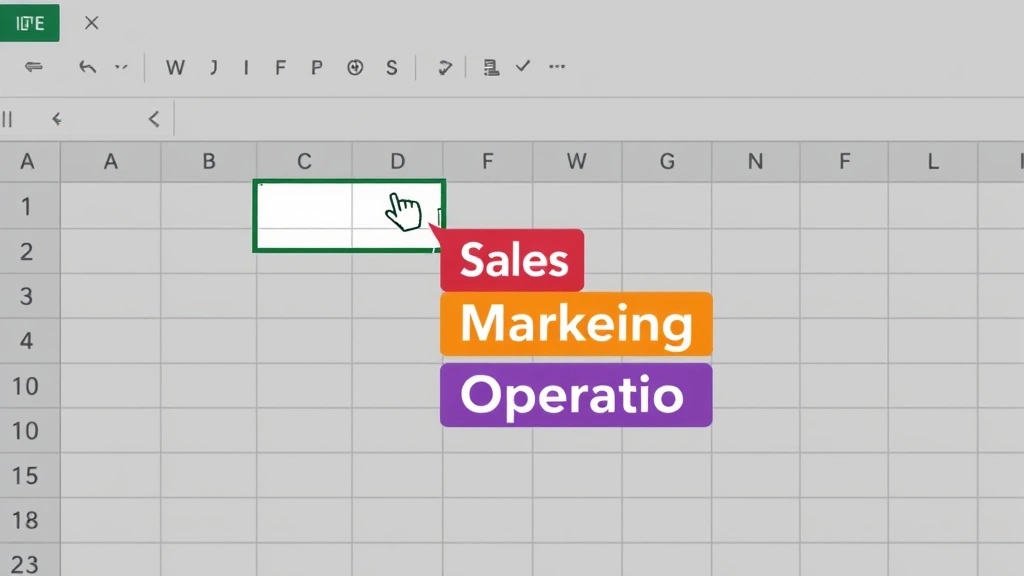
- Department names (Sales, Marketing, Operations, HR)
- Priority levels (High, Medium, Low)
- Status updates (Not Started, In Progress, On Hold, Complete)
- Product categories or SKUs
- Date ranges or time slots
- Geographic regions
You can also link drop-downs to cells in your spreadsheet, so if you update the list once, every drop-down that uses it updates automatically. This is where things get really powerful.
Step-by-Step Instructions: How to Make Drop Down List in Excel
Method 1: Simple List (Type Directly)
This is the fastest way if you have a short list and don’t plan to reuse it elsewhere.
- Select the cell (or cells) where you want the drop-down. Click on a single cell, or select a range. If you want the same drop-down in multiple cells, select them all at once (hold Ctrl and click, or click and drag).
- Go to the Data tab. In the ribbon, find the Data tab and click it.
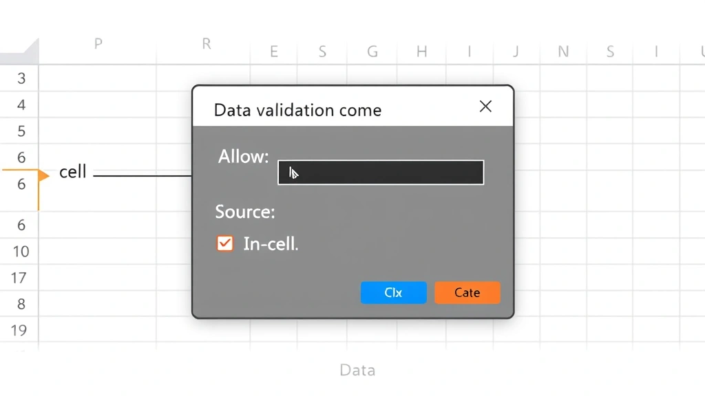
- Click Data Validation. You’ll see a button labeled “Data Validation” in the Data Tools group. Click the dropdown arrow next to it (not the main button—the small arrow).
- Select “Data Validation” from the menu. A dialog box opens. This is your control center.
- In the “Allow” dropdown, select “List.” This tells Excel you’re providing a specific list of options.
- In the “Source” field, type your options separated by commas. Example: “Red, Blue, Green, Yellow” or “Q1, Q2, Q3, Q4.” No spaces after commas unless you want them in your list.
- Leave “In-cell dropdown” checked. This shows the arrow users click to see the list.
- Click OK. You’re done. Test it by clicking the cell and seeing the arrow.
Pro tip: If your list has more than 5-10 items, this method gets tedious. Use Method 2 instead.
Method 2: List from Cells (The Smart Way)
This method links your drop-down to a range of cells in your spreadsheet. If you change the list, the drop-down updates automatically. This is how pros do it.
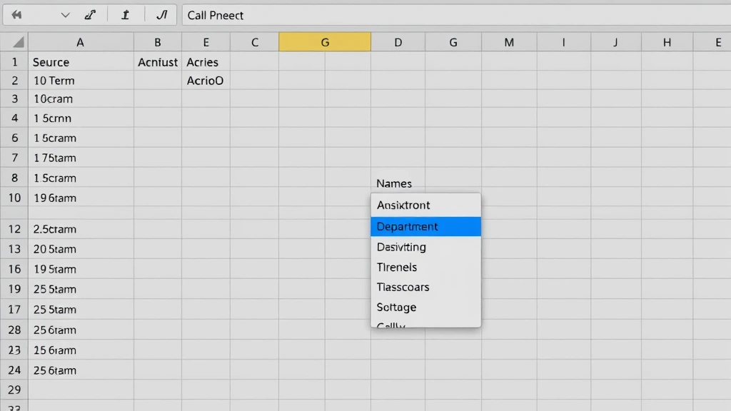
- Create your list in a column somewhere. Let’s say you put your options in column F, rows 1-5: Sales, Marketing, Operations, HR, Finance. Make sure there are no empty cells in the middle (Excel stops reading the list when it hits a blank).
- Select the cell where you want the drop-down. This could be in column A, row 2—wherever your data entry happens.
- Go to Data > Data Validation. (Data tab → Data Validation button → dropdown arrow)
- Set “Allow” to “List.”
- In the “Source” field, type the range of your list. If your list is in F1:F5, type: $F$1:$F$5. The dollar signs make it an absolute reference (it won’t change if you copy the formula).
- Check “In-cell dropdown” and click OK.
Now your drop-down pulls from those cells. If you add “Legal” to your list in F6 later, you’d need to update the validation range to $F$1:$F$6, but the concept is the same.
Using Named Ranges for Dynamic Lists
Here’s where how to make drop down list in Excel becomes genuinely elegant. Named ranges let you create a drop-down that automatically expands when you add new items to your list. No manual updates needed.
A named range is basically a nickname for a cell or range. Instead of saying “F1:F5,” you can say “Departments.” It’s cleaner, easier to read, and it can be dynamic.
Creating a Dynamic Named Range
- Put your list in a column. Let’s say it’s in F1:F100 (even though you only have 5 items now). Leave the rest blank.
- Go to Formulas > Define Name. (Or press Ctrl+F3 on Windows, Cmd+Fn+F3 on Mac.)
- In the “Name” field, type a name. Example: “Departments” (no spaces).
- In the “Refers to” field, use this formula:
=OFFSET($F$1,0,0,COUNTA($F$1:$F$100),1)This tells Excel: start at F1, count how many non-empty cells are in F1:F100, and make that your range. When you add a new department, the range expands automatically. - Click OK.
- Now create your drop-down using this named range. Go to Data Validation, set Allow to List, and in Source, type: Departments (just the name, no $ signs).
This is advanced stuff, but it saves hours of maintenance on large spreadsheets. You never have to think about updating the validation range again.
Advanced Techniques & Troubleshooting
Cascading Drop-Downs (Dependent Lists)
Sometimes you want one drop-down to control another. Example: select “Sales” in the first dropdown, and the second dropdown only shows salespeople. This is called a cascading or dependent drop-down, and it’s trickier but worth it for complex data.
The basic approach uses named ranges and INDIRECT formulas. If you have a list of departments and a list of employees under each department, you’d:
- Create separate named ranges for each department’s employees.
- In the second drop-down’s Source field, use: =INDIRECT(A1) where A1 contains the first drop-down. Excel then looks for a named range that matches whatever’s selected in A1.
This is beyond the scope here, but Microsoft’s guide on dependent drop-downs walks through it step-by-step.
Error Messages & Validation Rules
When someone tries to enter data that’s not on your list, you can show them a custom error message. Back in the Data Validation dialog:
- Click the “Error Alert” tab.
- Set “Style” to “Stop” (rejects invalid entries), “Warning” (warns but allows), or “Information” (just informs).
- Type a custom title and message. Example: Title: “Invalid Entry” Message: “Please select from the list provided.”
This prevents garbage data and guides users toward correct entries.
Troubleshooting Common Issues
Drop-down isn’t showing: Make sure “In-cell dropdown” is checked in the Data Validation dialog. Also, check that the cell isn’t formatted as text (format it as General first).
List isn’t updating when I change source cells: If you used a static range (like $F$1:$F$5), you have to manually update it. Use a named range with OFFSET formula instead.
Drop-down works but shows blank cells: Your source range has empty cells in the middle. Excel reads the list until it hits a blank, then stops. Remove blanks or restructure your list.
Can’t edit the list after creating the drop-down: Go back to Data Validation, update the Source field, and click OK. The drop-down updates instantly.
For more detailed troubleshooting, check Excel’s official support documentation, or consult community forums where users share workarounds.
Best Practices for Drop-Down Lists
Keep Lists Short and Clear
A drop-down with 50 options defeats the purpose. Users scroll forever, and you lose the consistency benefit. If you have a long list, consider using a lookup tool or filtering instead. Aim for 3-15 options per drop-down. If it’s longer, break it into categories (cascading drop-downs).
Label Your Lists
If your source cells are in column F, add a header in F1 that explains what the list is. “Departments,” “Status,” “Priority”—something clear. This helps you (and anyone else editing the spreadsheet) understand what’s what.
Protect Your Spreadsheet
Once you’ve built your drop-downs, protect the sheet so people can’t accidentally delete them or change the validation rules. You can also lock cells in Excel to prevent editing of source lists while allowing drop-down cells to be filled. Go to Review > Protect Sheet, set a password (optional), and choose what users can do.
Use Consistent Formatting
If drop-downs are in column A, put them all in column A. Don’t scatter them randomly. This makes your spreadsheet predictable and easier to use. You can also freeze rows in Excel to keep headers visible while users scroll, making it clear which column is which.
Document Your Choices
If someone else will use this spreadsheet, add a note or legend explaining what each option means. “High priority = must complete within 24 hours” is clearer than just “High.” Put this in a separate sheet or at the top of the main sheet.
Combine with Other Excel Features
Drop-downs work beautifully with other Excel tools. For example:
- Conditional formatting: Highlight cells with drop-downs in red if they say “Overdue,” green if “Complete.”
- COUNTIF formulas: Count how many items are marked “In Progress.” See how to check duplicates in Excel for related data-cleaning techniques.
- Pivot tables: Analyze drop-down data to see trends (e.g., which departments have the most high-priority items).
- Merged cells: If you’re building a form-like spreadsheet, you might merge two columns in Excel for labels, then put drop-downs next to them.
Frequently Asked Questions
Can I use a drop-down list in Excel Online or Google Sheets?
– Yes, but the steps differ slightly. In Excel Online, go to Data > Data Validation (same as desktop). Google Sheets uses Data > Validation, and the interface is similar but not identical. The core concept is the same everywhere.
What’s the maximum number of items in a drop-down list?
– Excel can handle thousands of items, but practically speaking, a drop-down with more than 20-30 options becomes unwieldy. Users won’t want to scroll through a huge list. Consider categories or a different approach (like a lookup table with filtering) for large datasets.
Can I have drop-downs that change based on another cell’s value?
– Yes, this is a cascading or dependent drop-down. It requires named ranges and the INDIRECT function. It’s more advanced, but Microsoft’s tutorial covers it thoroughly.
How do I copy a drop-down to other cells?
– Select the cell with the drop-down, copy it (Ctrl+C), select the range where you want to paste it, and paste (Ctrl+V). The validation rules copy over. If you used a relative reference, it adjusts; if you used absolute references (with $), it stays the same.
What happens if I delete the source list?
– If you delete the cells your drop-down references, the drop-down breaks. Users see an error or the list disappears. Always keep your source list intact, or use a protected sheet so people can’t accidentally delete it.
Can I make a drop-down that allows multiple selections?
– Not with native Excel data validation. A single drop-down cell can only hold one value. If you need multiple selections, you’d need VBA (macros) or a workaround like separate cells for each selection. For most purposes, one selection per cell is the standard.
Is there a way to make drop-downs look fancier or more visible?
– You can use conditional formatting to highlight cells with drop-downs, or add background colors to make them stand out. You can also use freeze cells in Excel techniques to keep drop-down sections visible. Functionally, the drop-down itself is simple, but you can make the surrounding design cleaner.
Can I use formulas inside a drop-down list?
– Not directly in the Source field. But you can use formulas to generate your source list in cells, then reference those cells in the drop-down. For example, use a formula to pull unique values from a database, then make a drop-down from those cells.


