How to Freeze Panes in Excel: Easy & Essential Guide

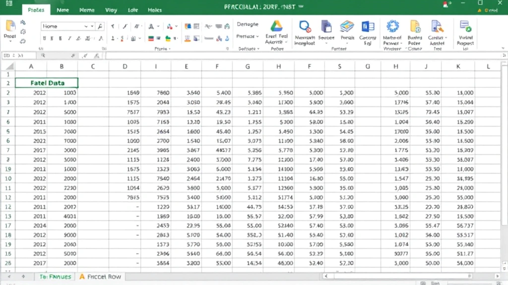
Working with large spreadsheets in Excel can be frustrating when you scroll and lose sight of your headers. Learning how to freeze panes in Excel is one of the most practical skills that saves time and prevents data entry errors. Whether you’re managing financial reports, inventory lists, or project timelines, freezing panes keeps your column and row headers visible while you navigate through thousands of rows of data.
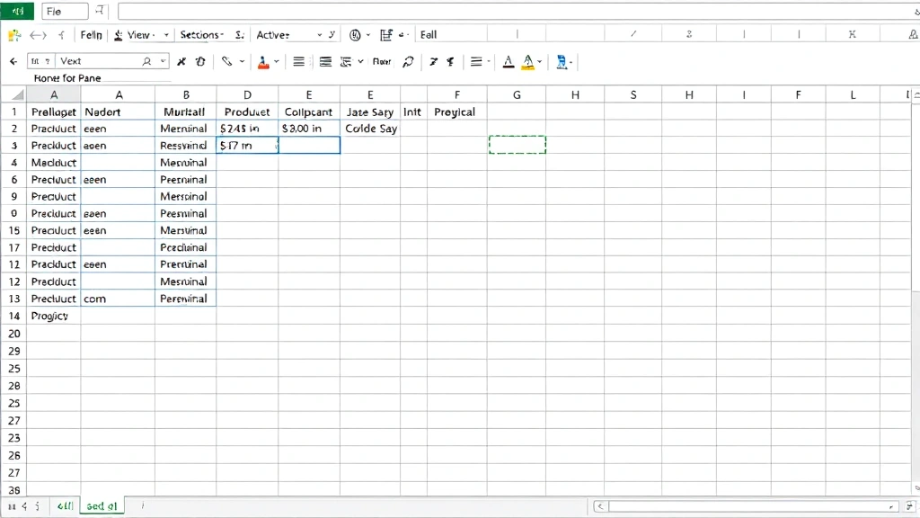
Quick Answer: To freeze panes in Excel, select the cell below the row and to the right of the column you want to freeze, then go to the View tab and click Freeze Panes. For example, to freeze the first row, click cell A2, then select Freeze Panes. To freeze both the first row and first column, click cell B2 before freezing. This feature works identically across Windows and Mac versions of Excel.
Tools & Materials Needed
- Microsoft Excel (2016 or later, or Office 365)
- A spreadsheet with headers or data you want to keep visible
- Mouse or trackpad for navigation
- Basic understanding of Excel interface
Why Freeze Panes in Excel Matters
Understanding why you should freeze panes in Excel helps you work more efficiently with data. When you have a spreadsheet with dozens of columns and hundreds of rows, scrolling horizontally or vertically causes your headers to disappear. This makes it nearly impossible to remember which column contains what information or which row you’re currently editing.
Freezing panes solves this problem by keeping designated rows and columns visible at all times, regardless of where you scroll. According to WikiHow’s comprehensive Excel guides, this feature is essential for professional data management. The benefits include reduced data entry errors, improved workflow speed, and better overall spreadsheet navigation. Financial analysts, project managers, and data entry specialists rely on this feature daily to maintain accuracy and efficiency.
Real-world applications include tracking inventory across multiple warehouses, managing employee timesheets, analyzing sales data by region, and maintaining budget spreadsheets. Once you master how to freeze panes in Excel, you’ll wonder how you ever worked without it.
How to Freeze the First Row
Freezing the first row is the most common use case and the easiest to master. This technique keeps your column headers visible while you scroll through data below. Start by opening your Excel spreadsheet with headers in the first row. Make sure your cursor is positioned in the spreadsheet area, not in a cell being edited.
Step-by-step instructions:
- Click on any cell in the second row (row 2) of your spreadsheet
- Navigate to the View tab in the Excel ribbon menu
- Click the Freeze Panes button (it shows a window icon with lines)
- A thin line will appear below row 1, indicating the freeze is active
- Scroll down to verify your headers remain visible
The key principle here is that Excel freezes everything above and to the left of your selected cell. By clicking cell A2, you’re telling Excel to freeze everything in row 1. This applies to all columns simultaneously, making it perfect for spreadsheets with multiple data columns and a single header row.

How to Freeze Columns in Excel
Sometimes you need to keep row identifiers visible while scrolling right through many columns of data. How to freeze panes in Excel for columns follows the same principle but with horizontal positioning. This is particularly useful for spreadsheets tracking multiple years, quarters, or product categories across columns.
Freezing the first column:
- Click on any cell in the second column (column B)
- Go to the View tab
- Select Freeze Panes
- A vertical line appears to the right of column A
- Scroll right to confirm column A stays visible
You can also freeze multiple columns using the same method. If you want to freeze the first three columns, click on any cell in column D (the fourth column), then apply Freeze Panes. The principle remains consistent: Excel freezes everything to the left of your selected cell.
As reviewed by Family Handyman’s practical guides, mastering these basic techniques forms the foundation for advanced spreadsheet work. Whether you’re managing a parts inventory with product codes in columns A-C or tracking monthly expenses across multiple columns, freezing columns keeps your reference data always accessible.
Freezing Both Rows and Columns
The most powerful use of how to freeze panes in Excel involves freezing both rows and columns simultaneously. This creates a frozen quadrant in the top-left corner while allowing you to scroll freely through data in all directions. Financial analysts and data scientists use this technique constantly when working with complex datasets.
Complete freezing process:
- Identify which row and column you want as your last frozen pane
- Click on the cell that is one row below and one column to the right of your freeze point
- For example, to freeze row 1 and columns A-B, click cell C2
- Navigate to View tab and click Freeze Panes
- Both a horizontal and vertical line appear, creating four quadrants
- Test by scrolling both horizontally and vertically
This technique is invaluable for complex spreadsheets. Imagine a sales report with months across columns (January, February, March, etc.) and product names down rows. By freezing both, you see product names and month headers regardless of scroll position. The frozen quadrant approach ensures you never lose context while analyzing data.
How to Unfreeze Panes
Removing frozen panes is just as simple as creating them. If you need to adjust your freeze settings or work with the spreadsheet in a different way, unfreezing takes seconds. Understanding how to freeze panes in Excel also means knowing when to turn it off.
Unfreezing steps:
- Go to the View tab in the ribbon
- Click Freeze Panes again
- Select Unfreeze Panes from the dropdown menu
- All frozen lines disappear immediately
- Your spreadsheet returns to normal scrolling behavior
Some users prefer to unfreeze, adjust their data layout, and then refreeze with new settings. Others might unfreeze temporarily to copy entire columns or rows without restrictions. The flexibility of toggling freeze panes on and off makes Excel more adaptable to different tasks.
Troubleshooting Common Issues
Even experienced users encounter problems with how to freeze panes in Excel. Understanding common issues helps you resolve them quickly and maintain productivity. Most problems stem from misunderstanding the selection mechanics or confusion about which cell to click.
Problem: Freeze Panes button is grayed out
This typically means you’re not in the right view mode. Excel’s Freeze Panes feature only works in Normal view. If you’re in Page Break Preview or other views, the button appears disabled. Switch to View tab and select Normal to enable the feature. Additionally, ensure you’re not in edit mode within a cell—click elsewhere in the spreadsheet first.
Problem: Wrong rows or columns are frozen
This is the most common mistake. Remember that Excel freezes everything above and to the left of your selected cell. If you want to freeze rows 1-3, click cell A4, not A3. If you want columns A-C frozen, click cell D1. The selected cell itself is never frozen; only what’s above and to its left.
Problem: Freeze Panes not working after applying filters
Filters and freeze panes sometimes conflict. If you applied AutoFilter after freezing, try unfreezing first, applying filters, then refreezing. Alternatively, freeze panes before applying filters to avoid compatibility issues. According to HowStuffWorks’ technology section, this sequencing prevents most Excel feature conflicts.
Problem: Frozen panes disappear when sharing the file
If you share your Excel file and the recipient doesn’t see frozen panes, ensure you saved the file after applying the freeze. Excel saves freeze pane settings within the file, but only if you explicitly save after making changes. Save the file in .xlsx format for maximum compatibility across different Excel versions.
Advanced Freezing Techniques
Once you master basic how to freeze panes in Excel techniques, explore advanced applications that enhance your spreadsheet skills. These methods work with other Excel features to create powerful data analysis tools.
Combining Freeze Panes with Data Validation: You can use drop-down lists in Excel alongside frozen headers for better data entry. Freeze your header row, then add drop-down validation to data columns below. Users can scroll through data while always seeing what each column represents.
Freezing with Conditional Formatting: When you freeze panes and apply conditional formatting, the visual indicators remain visible. This combination helps identify important data points while maintaining header visibility. For example, freeze your product names and dates, then apply color formatting to highlight overdue items.
Using Freeze Panes with Sorting and Filtering: Always freeze panes before applying sorts or filters. This ensures your headers remain visible and locked in place while your data reorganizes. If you need to find duplicates in Excel, frozen headers help you understand which columns you’re analyzing.
Freezing Multiple Sections: For extremely large spreadsheets, you might freeze a middle section. Click a cell in the middle of your data, then freeze. This keeps both top headers and left identifiers visible while scrolling through the core data area. This advanced technique suits complex financial models or scientific datasets.
Combining with Text Wrapping: If you have long header text, consider using text wrapping in Excel before freezing. This ensures your headers display completely while remaining frozen. Adjust row height for wrapped headers before freezing to maintain optimal visibility.
Protecting Frozen Panes: For shared workbooks, you might want to lock cells in Excel to prevent accidental unfreezing. This combines protection features with freeze panes, ensuring your carefully organized spreadsheet layout remains stable when others access it.
As noted by The Spruce’s how-to resources, mastering these combinations transforms you into an advanced Excel user capable of creating professional, user-friendly spreadsheets.
FAQ
Can I freeze panes in Excel on a Mac?
Yes, the process is identical on Mac and Windows versions of Excel. Go to View tab, click Freeze Panes, and select your option. The interface looks slightly different on Mac, but the functionality remains the same.
What’s the difference between Freeze Panes and Freeze Rows/Columns?
In newer Excel versions, you’ll see separate options: “Freeze Panes,” “Freeze Top Row,” and “Freeze First Column.” The latter two are shortcuts for common scenarios. Freeze Panes is more flexible, allowing you to freeze any combination of rows and columns by selecting the appropriate cell first.
Will frozen panes print on my document?
No, frozen panes are a view-only feature. They won’t appear in printed output or PDFs. If you want headers to repeat on every printed page, use the “Print Titles” feature in Page Layout instead of Freeze Panes.
Can I freeze panes in Excel Online?
Yes, Excel Online supports freeze panes functionality. The steps are the same: select your cell, go to View, and choose Freeze Panes. This works seamlessly across desktop and browser versions.
Why does my freeze pane line disappear sometimes?
If you unintentionally click Freeze Panes again, it toggles off. Also, switching between different view modes can temporarily hide the freeze line. Switch back to Normal view and verify your freeze is still active by scrolling.
Can I have multiple freeze pane sections?
Excel only allows one freeze pane configuration per sheet. You can freeze one row, one column, or one combination of rows and columns, but not multiple separate sections. If you need multiple frozen areas, consider using separate worksheets or splitting the window instead.
How do I freeze panes in a specific area of my spreadsheet?
Click the cell at the intersection point where you want freezing to begin. Everything above and to the left of that cell will freeze. For example, to freeze rows 1-5 and columns A-D, click cell E6, then apply Freeze Panes.
Does freezing panes affect data calculations?
No, freezing panes is purely a visual feature. It doesn’t change any formulas, values, or calculations in your spreadsheet. It only controls what you see on screen.
Mastering how to freeze panes in Excel transforms your spreadsheet experience from frustrating to efficient. Whether you’re managing a small inventory list or analyzing complex financial data, this essential feature keeps your headers visible and your workflow smooth. Start with freezing a single row, progress to freezing both rows and columns, and soon you’ll be navigating large datasets with confidence and precision.


