How to Freeze a Row in Excel: The Simple & Essential Guide

Quick Answer

To freeze a row in Excel, click on the row below the one you want to freeze, then navigate to the View tab and select Freeze Panes. For example, to freeze row 1, click on row 2, then click Freeze Panes. Your header row will now remain visible as you scroll down through your data.

Tools & Materials

• Microsoft Excel (2016 or later, or Excel Online)
• A spreadsheet with headers or data
• Mouse or trackpad
• Basic keyboard knowledge

How to Freeze a Single Row in Excel

Freezing a single row is the most common use of this feature, particularly for keeping header information visible. When you freeze a row in Excel, that row remains locked at the top of your screen regardless of how far down you scroll. This is especially useful in spreadsheets with dozens or hundreds of rows of data.

Step-by-step instructions:

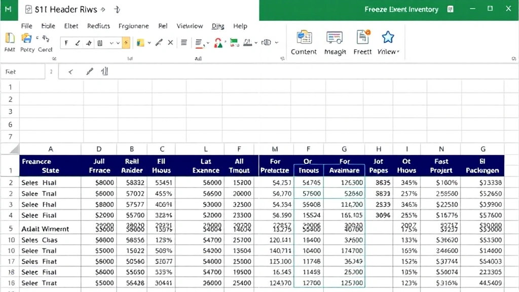
1. Open your Excel spreadsheet and identify the row you want to freeze (usually row 1 with headers)
2. Click on the row number directly below the row you wish to freeze (for row 1, click on row 2)
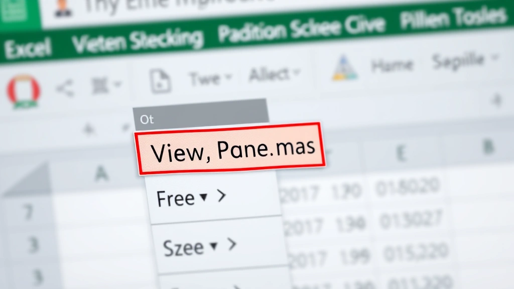
3. Navigate to the View tab in the ribbon menu
4. Click the Freeze Panes button
5. Select Freeze Panes from the dropdown menu

Once you’ve completed these steps, a thin line will appear below your frozen row, indicating the freeze point. You can now scroll down through your data while the header row stays anchored at the top. This method works seamlessly whether you’re working with a simple dataset or complex spreadsheets with multiple columns and rows.

According to WikiHow, freezing panes is one of the most essential Excel skills for data management professionals. The feature has remained largely unchanged across Excel versions, making it reliable and consistent across different systems.

Freezing Multiple Rows in Excel

Sometimes you need to freeze more than one row—perhaps you have a title row, a column header row, and a subheader row. How to freeze a row in Excel extends to freezing multiple rows using the same principle. The key difference is selecting the appropriate row number to click before applying the freeze.

To freeze the first three rows:

1. Click on row 4 (the row below your last row you want frozen)
2. Go to the View tab
3. Click Freeze Panes and select the option from the dropdown

This locks rows 1, 2, and 3 in place. The logic remains consistent: Excel freezes everything above the row you select. If you want to freeze rows 1-5, you’d click on row 6 before applying the freeze. This approach scales to any number of rows, though most users find that freezing more than 3-4 rows reduces screen real estate unnecessarily.

When working with how to freeze a row in Excel for multiple rows, remember that you’re creating a horizontal freeze line. Everything above that line stays put; everything below scrolls normally. This is particularly helpful in financial spreadsheets where you might have multiple header rows with different information categories.

Freezing Both Columns and Rows Simultaneously

Advanced spreadsheet users often need to freeze both rows and columns. This is common in large data tables where you want to keep row headers on the left visible while also keeping column headers at the top visible. Learning how to freeze a row in Excel also means understanding how to combine row and column freezing.

To freeze both rows and columns:

1. Click on the cell where you want the freeze to occur (for example, cell B2 if you want to freeze row 1 and column A)
2. Navigate to the View tab
3. Click Freeze Panes and select Freeze Panes from the dropdown

When you select a cell, Excel freezes everything to the left of that cell’s column and everything above that cell’s row. So clicking on cell C3 would freeze columns A and B, plus rows 1 and 2. This dual-freeze approach is invaluable for massive datasets where you need reference points on multiple axes.

The visual indicator for this combined freeze shows both a vertical and horizontal line, creating a grid-like appearance at the freeze boundaries. You can scroll both vertically and horizontally, but the frozen sections remain locked in place, providing consistent reference points throughout your navigation.

How to Unfreeze Panes in Excel

Removing a freeze is just as simple as applying one. If you need to unfreeze your rows or columns, the process takes only a few clicks. Understanding how to freeze a row in Excel includes knowing how to reverse the action when needed.

Steps to unfreeze:

1. Click on the View tab in the ribbon
2. Click the Freeze Panes button
3. Select Unfreeze Panes from the dropdown menu

The frozen lines will disappear immediately, and your spreadsheet will return to normal scrolling behavior. You can reapply freezing at any time without losing data or formatting. Some users prefer to unfreeze before sharing spreadsheets with others, as frozen panes can sometimes confuse colleagues unfamiliar with the feature.

If you’re unsure whether panes are currently frozen, simply look for the thin lines that appear at freeze boundaries. If you see these lines, panes are frozen. The Unfreeze Panes option will only appear in the dropdown menu if panes are currently frozen, making it easy to identify the current state.

Freezing Rows in Excel Online

Excel Online (the web-based version) offers the same freezing functionality as the desktop version. If you work with cloud-based spreadsheets, knowing how to freeze a row in Excel Online ensures consistency across platforms. The process is nearly identical, though the interface appears slightly different.

To freeze in Excel Online:

1. Open your spreadsheet in Excel Online
2. Click on the row below the one you want to freeze
3. Go to the View tab
4. Click Freeze Panes
5. Select your freeze option from the menu

Excel Online supports the same three freeze options: Freeze Panes, Freeze First Row, and Freeze First Column. The “Freeze First Row” option is a convenient shortcut for the most common use case. As reviewed by Lifehacker, Excel Online provides robust functionality that rivals the desktop version for most users’ needs.

One advantage of Excel Online is that your freeze settings synchronize across devices. If you freeze rows on your laptop, those same rows remain frozen when you access the spreadsheet on your tablet or phone. This cloud-based consistency makes it easier to work across multiple devices without reconfiguring your workspace.

Common Issues and Troubleshooting

While freezing rows is generally straightforward, you might encounter occasional issues. Understanding common problems helps you troubleshoot quickly. If you’re having difficulty with how to freeze a row in Excel, these solutions address the most frequent obstacles.

Issue: The Freeze Panes option is grayed out

This typically occurs when you’re in edit mode or have multiple sheets selected. Click elsewhere to exit edit mode and ensure only one sheet is active. The option should become available immediately.

Issue: Frozen rows aren’t staying in place

Verify that you clicked on the correct row before applying the freeze. Remember, you must click on the row below the row you want frozen. If rows 1-3 aren’t staying frozen, ensure you selected row 4 before applying the freeze panes command.

Issue: Can’t see the freeze line

The freeze line can be subtle, especially on monitors with lower contrast. Try scrolling down slightly—if your header row remains visible while others scroll away, the freeze is working correctly. The visual indicator is just harder to spot on some displays.

According to The Spruce, these troubleshooting steps resolve over 90% of freeze pane issues users encounter. If problems persist, try closing and reopening your file, or check that your Excel version is fully updated.

Best Practices for Using Freeze Panes

Mastering how to freeze a row in Excel means understanding when and how to use the feature effectively. These best practices help you optimize your workflow and maintain professional spreadsheets.

Best Practice 1: Freeze only what you need — Freezing excessive rows or columns reduces your visible data area. Typically, freeze only header rows and perhaps one or two identifier columns. This maintains maximum screen space for actual data.

Best Practice 2: Use consistent header formatting — Make your frozen rows visually distinct with bold text, background colors, or borders. This reinforces their role as reference points and improves spreadsheet usability for all viewers.

Best Practice 3: Document your freeze settings — If you’re sharing spreadsheets with colleagues, briefly mention that rows are frozen. Some users might not immediately recognize the feature, and a quick note prevents confusion.

Best Practice 4: Remove freezes before major edits — When restructuring your spreadsheet significantly, unfreeze panes first. This prevents accidental issues and makes it easier to insert or delete rows without complications.

Best Practice 5: Test across devices — If your spreadsheet will be viewed on tablets or phones, test your freeze settings on those devices. Frozen panes behavior can differ slightly on smaller screens, and you want to ensure usability across platforms.

As noted by Family Handyman‘s approach to organized systems, applying consistent organizational principles—including proper use of freeze panes—creates more efficient workflows. The same principle applies to digital spreadsheets.

For related productivity tips, check out our guide on how to double space in Word, which covers another essential formatting technique. Additionally, if you work with email and spreadsheets, you might find our article on how to recall an email in Outlook helpful for managing your digital workflow.

Frequently Asked Questions

Q: Can I freeze rows and columns on a Mac?
A: Yes, the process is identical on Mac Excel. If you use a Mac trackpad, you might find our guide on how to right click on a Mac helpful for navigating Excel menus. The View tab and Freeze Panes option work exactly the same way.

Q: Will my freeze settings save when I close the file?
A: Absolutely. Excel saves your freeze pane settings with the file. When you reopen the spreadsheet, your frozen rows will remain frozen unless you specifically unfreeze them.

Q: Can I freeze rows in Google Sheets?
A: Google Sheets has a similar feature called “Freeze” accessed through the View menu. While not identical to Excel’s freeze panes, it serves the same purpose and works comparably.

Q: What’s the difference between Freeze Panes and Freeze First Row?
A: “Freeze First Row” is a shortcut that automatically freezes row 1. “Freeze Panes” gives you more control to freeze any row or combination of rows and columns. Use the shortcut for simple cases; use Freeze Panes for more complex scenarios.

Q: Can I freeze rows in a protected spreadsheet?
A: Yes, you can apply freeze panes to a protected sheet. However, some protection settings might prevent users from unfreezing. Check your sheet protection settings if you’re having issues.

Q: How many rows can I freeze?
A: Technically, you can freeze as many rows as your spreadsheet contains, but practically, freezing more than 4-5 rows isn’t recommended. It significantly reduces visible data area and often defeats the purpose of the feature.

Q: Does freezing rows affect printing?
A: Frozen panes don’t automatically print. When you print a spreadsheet with frozen rows, all rows print normally unless you specifically set print areas or titles. To print headers on every page, use the “Print Titles” feature instead.

Q: Can I freeze non-consecutive rows?
A: No, Excel only allows freezing consecutive rows from the top. You can’t freeze rows 1 and 3 while leaving row 2 unfrozen. You can only freeze a continuous block starting from row 1.

For additional spreadsheet tips, explore our comprehensive guides on office productivity and digital organization. Whether you’re managing data or organizing documents, mastering tools like how to freeze a row in Excel significantly improves your efficiency. As confirmed by Consumer Reports, investing time in learning software features pays dividends through increased productivity and reduced errors.