How to Freeze a Column in Excel: Essential & Easy Guide

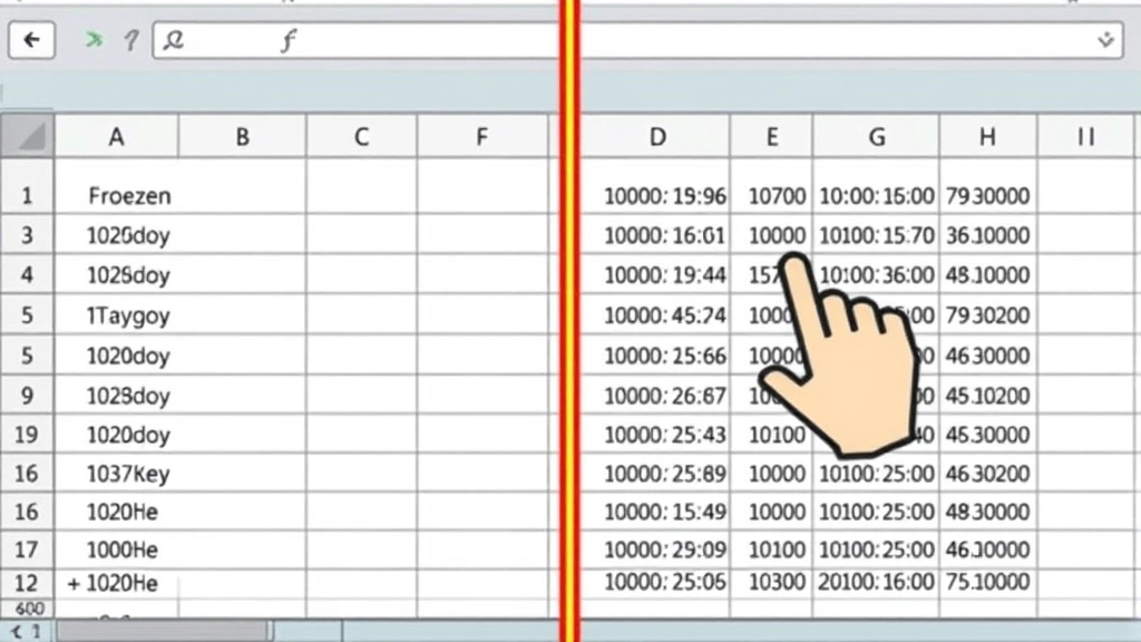
You’re staring at a massive spreadsheet with hundreds of rows, and you scroll down—suddenly, the column headers disappear. You have no idea what data you’re looking at anymore. Sound familiar? That’s the exact problem freezing columns solves. Learning how to freeze a column in Excel is one of those skills that seems small until you realize it saves you hours of frustration. Whether you’re managing inventory, tracking sales, or organizing any dataset, freezing columns keeps your reference data visible no matter how far you scroll.

The good news? It takes about 30 seconds once you know where to click. No formulas. No complicated steps. Just a straightforward feature built into Excel that most people never discover.

What Does Freezing a Column Actually Do?

Think of freezing a column like anchoring a reference point on a map. When you freeze a column in Excel, that column stays visible on your screen even when you scroll horizontally to the right. The rest of your spreadsheet moves, but the frozen column remains locked in place.

Here’s why this matters: Imagine you have a spreadsheet with 50 columns of data. Column A contains customer names. Columns B through Z contain monthly sales data for the past two years. Without freezing, you’d scroll right to see January’s data, and suddenly Column A (the customer names) would vanish off-screen. You’d be looking at numbers with no context. Freeze Column A, and it stays put while you navigate all the way to December without losing track of whose data you’re viewing.

This applies to rows too—you can freeze header rows so they stay visible when scrolling down through thousands of entries. But this guide focuses specifically on how to freeze a column in Excel, which is slightly different from freezing rows (though you can do both simultaneously, which we’ll cover later).

Pro Tip: Freezing doesn’t lock cells or prevent editing. It’s purely visual. You can still edit frozen cells normally—they just stay on-screen while you work.

How to Freeze a Single Column (Step-by-Step)

This is the most common scenario. You want Column A (or any single column) to stay visible while you scroll through the rest of your data.

1. Click on the column header to the right of the column you want to freeze. If you want to freeze Column A, click on Column B’s header. If you want to freeze Column C, click on Column D’s header. This tells Excel: “Everything to the left of this point should stay frozen.”
2. Go to the View tab at the top of the ribbon in Excel.
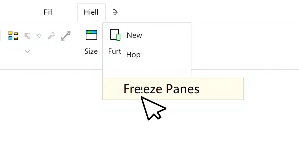
3. Click “Freeze Panes” (or “Freeze” in newer Excel versions). A dropdown menu appears.
4. Select “Freeze Panes” from the dropdown.
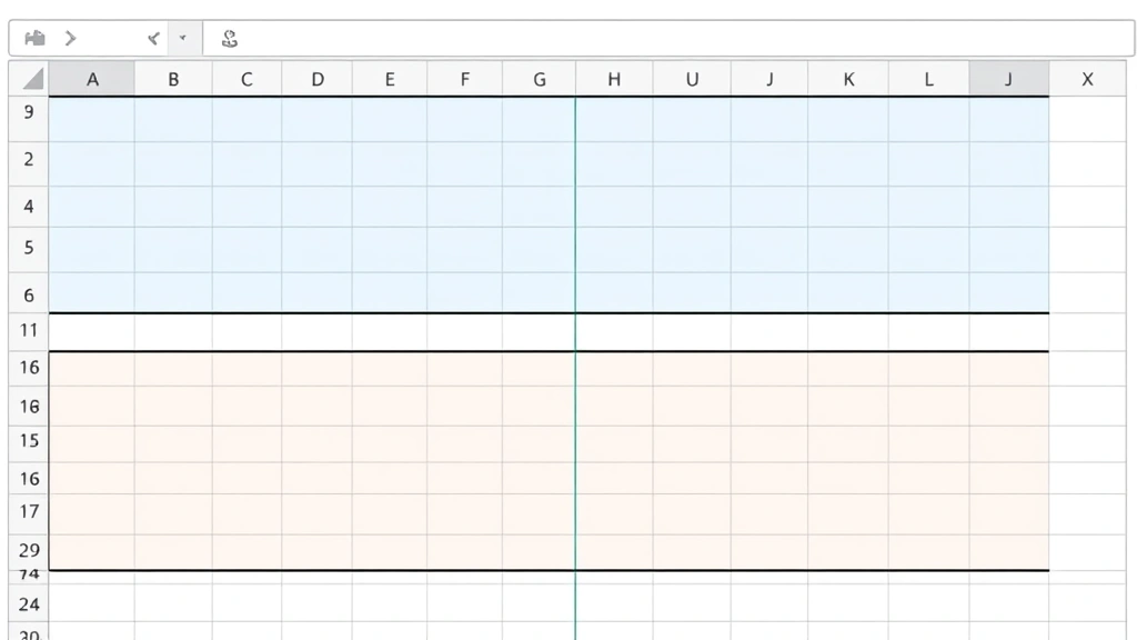
5. You’re done. A thin black line should appear between the frozen and unfrozen columns. Scroll right, and watch your frozen column stay put.

That’s it. Seriously. The black line is your visual confirmation that the freeze is active. If you don’t see it, the freeze didn’t take. Go back and try again—usually it means you clicked the wrong column header.

Let’s say you’re working with a customer database where Column A has names, Column B has IDs, and Columns C through Z have contact info and notes. You’d click on Column C’s header, then View → Freeze Panes. Now Columns A and B stay visible while you scroll through all the contact data.

Safety Warning: Make sure you’re clicking the column header (the letter at the very top), not a cell within the column. The header is the clickable area that selects the entire column.

Freezing Multiple Columns at Once

What if you need to freeze more than one column? Same process, just adjust where you click.

1. Identify how many columns you want to freeze. Let’s say you want to freeze Columns A, B, and C (three columns total).
2. Click on Column D’s header. You’re telling Excel to freeze everything to the left of Column D.
3. Go to View → Freeze Panes → Freeze Panes.
4. Columns A, B, and C are now frozen. Scroll right, and all three stay visible.

The pattern is always the same: click the column header immediately to the right of your last frozen column, then freeze. If you want to freeze five columns, click Column F’s header. Ten columns? Click Column K’s header.

This is particularly useful for large datasets where you have multiple reference columns at the start. For example, in a project management spreadsheet, you might freeze columns for Project Name, Project Manager, Start Date, and Status—then scroll through dozens of columns tracking individual task details.

Freezing Both Rows and Columns Together

Here’s where it gets powerful. You can freeze both rows AND columns simultaneously. This is essential for spreadsheets with headers on top and reference data in the leftmost columns.

Let’s say your spreadsheet has:

• Row 1: Column headers (Month, Year, Product, Sales, etc.)
• Column A: Product names
• Column B: Product IDs
• Data starts in cell C2

You want Row 1 to stay visible when scrolling down, AND Columns A-B to stay visible when scrolling right. Here’s how:

1. Click on the cell where your unfrozen data begins. In this example, click on cell C2 (the intersection point below Row 1 and to the right of Column B).
2. Go to View → Freeze Panes → Freeze Panes.
3. Everything is now frozen. Row 1 stays at the top, Columns A-B stay on the left, and you can scroll through the data freely.

This is the most versatile freezing setup for professional spreadsheets. When you click on the cell where your actual data starts (not a column header, not a row header—the first cell of your data), Excel freezes everything above and to the left of that point.

Pro Tip: If your spreadsheet has multiple header rows (Row 1 and Row 2, for example), click the cell in the first row of actual data. If headers are in Rows 1-2 and data starts in Row 3, click on a cell in Row 3.

How to Unfreeze Columns

Changed your mind? Unfreezing is just as simple.

1. Go to View → Freeze Panes.
2. Click “Unfreeze Panes.”
3. The black line disappears, and your columns are unfrozen.

That’s all. No columns are harmed in the process. Everything stays exactly where it was—you’re just removing the freeze lock.

One important note: you can only have one freeze active at a time. If you freeze columns and then freeze different columns later, the new freeze replaces the old one. You can’t have Column A frozen and also Column M frozen independently. The freeze always works from the left edge or top edge of your data.

Troubleshooting Common Freezing Problems

This usually means you’re on a protected sheet or you’re in a special view mode. Check if the sheet is password-protected (you can learn more about this in our guide on how to password protect an Excel file). If it is, you’ll need the password to unprotect it before freezing. Also make sure you’re not in Page Preview or any other special view.

You probably didn’t click the right column header. Remember: click the column header to the RIGHT of the column you want frozen. If you want Column A frozen, click Column B. If nothing happened, try clicking View → Freeze Panes again—sometimes Excel needs a moment to register.

The line is subtle in some Excel themes. It’s usually there even if you can’t see it clearly. Test by scrolling right—if your columns stay put, the freeze is working. The visual indicator is just hard to spot sometimes. You can also check by going back to View → Freeze Panes. If “Unfreeze Panes” is the option (instead of “Freeze Panes”), you have an active freeze.

No problem. Go to View → Freeze Panes → Unfreeze Panes, then start over. There’s no penalty for unfreezing and re-freezing.

Freezing can behave oddly in shared workbooks or when the file is in compatibility mode. If you’re working with an older Excel file (.xls instead of .xlsx), try saving it as a modern format first. According to Microsoft’s support documentation, some features work better in newer file formats.

Pro Tips for Power Users

When you freeze cells in Excel, you can also apply AutoFilter to your headers. Freeze Row 1 and Columns A-B, then add filters to Row 1. Now you can filter your data while keeping your reference columns visible. This is incredibly powerful for large datasets.

Frozen columns work perfectly with color-coded data. Freeze your reference columns, then use conditional formatting on the rest of your data. The frozen columns stay visible while the formatted data scrolls by, giving you constant context for what you’re viewing.

The steps here work for Excel on Windows and Mac. In Excel Online (web version), the process is identical—View → Freeze Panes. In Google Sheets, it’s slightly different (Format → Freeze), but the concept is the same. If you’re working across platforms, the principle is universal: click where your data starts, then freeze.

Here’s something many people don’t realize: frozen panes don’t automatically print the way they appear on-screen. If you print a spreadsheet with frozen columns, those columns might not repeat on every page. To get frozen columns to repeat on printouts, you need to set print titles separately under Page Layout → Print Titles. This is a different feature than freezing, but it solves the same problem for printed documents.

Freezing doesn’t slow down your spreadsheet. It’s a view setting, not a formula or calculation. Even with thousands of rows and dozens of frozen columns, freezing has zero performance impact. Use it liberally.

You can add columns in Excel without affecting your freeze settings. The freeze stays active. Similarly, if you need to combine two cells in Excel, the freeze won’t interfere. You can also add a drop down list in Excel in frozen columns without issues. Freezing is a non-destructive view setting that plays nicely with other features.

Frequently Asked Questions

Can I freeze columns and rows at the same time?

– Yes. Click on the cell where your actual data starts (not in a header row or reference column), then go to View → Freeze Panes. Everything above and to the left of that cell will freeze.

What’s the difference between freezing and splitting?

– Splitting (View → Split) creates two independent scrollable panes. Freezing locks certain columns or rows in place. Freezing is usually what you want. Splitting is useful if you want to compare two different parts of the same spreadsheet side-by-side.

Does freezing protect my data?

– No. Freezing is purely visual. It doesn’t lock cells or prevent editing. If you want to protect data, you need to use sheet protection (Format → Cells → Protection, then Tools → Protect Sheet).

Can I freeze non-adjacent columns?

– No. Freezing always works from the left edge. You can only freeze continuous columns starting from Column A. You can’t freeze Column A and Column C while leaving Column B unfrozen.

Will my freeze settings save when I close the file?

– Yes. Excel saves freeze settings with the file. When you reopen the spreadsheet, your frozen columns will still be frozen. This is stored in the file itself, not just in your current session.

How do I know if a spreadsheet has frozen columns?

– Look for a thin black (or colored) line separating the frozen and unfrozen areas. You can also go to View → Freeze Panes. If “Unfreeze Panes” is available (instead of “Freeze Panes”), there’s an active freeze.

Can I freeze columns in Excel formulas or pivot tables?

– Yes. Freezing works on any worksheet, including those with formulas, pivot tables, or other complex structures. It’s a view setting, not a data setting.

What if I’m working on a Mac?

– The process is identical. View → Freeze Panes → Freeze Panes. Mac Excel has the same features as Windows Excel.

Can I adjust how many columns are frozen without unfreezing?

– No. You have to unfreeze first, then freeze again with a different column selected. There’s no “adjust freeze” option—you unfreeze and start over.

Does freezing work in Excel Online?

– Yes. Excel Online has the same freeze functionality. View → Freeze Panes works the same way. According to Microsoft Office support, most core features are available in the web version.

Why would I freeze columns instead of just scrolling?

– Freezing saves time and prevents confusion. Instead of constantly scrolling back to see your reference columns, they stay visible. For large spreadsheets with dozens or hundreds of columns, this is a massive productivity gain.

Can I freeze columns in a shared Excel file?

– Yes, but behavior can be unpredictable in shared workbooks. Each user’s freeze settings are independent. If you’re collaborating with others, consider documenting your freeze setup so everyone uses the same layout.