How to Create a Dropdown in Excel: Simple & Essential Guide

Dropdowns in Excel are one of the most powerful data validation features available, yet many users don’t realize how easy they are to create. Whether you’re building a professional spreadsheet for your team or organizing personal data, knowing how to create a dropdown in Excel will save you time and reduce data entry errors. This guide walks you through every method, from basic lists to advanced conditional dropdowns.

Tools & Materials You’ll Need

• Microsoft Excel (2016 or newer, or Excel Online)
• A list of items for your dropdown (can be in the same sheet or another sheet)
• Basic knowledge of cell references (A1, B2:B10, etc.)
• Optional: Named ranges for more advanced dropdowns
• Optional: Conditional formatting knowledge for dependent dropdowns

Creating a Basic Dropdown List

The simplest way to create a dropdown in Excel is by typing your items directly into the Data Validation dialog. This method works perfectly for small lists with 5-10 items that rarely change.

Step 1: Select Your Target Cell Click on the cell where you want the dropdown to appear. If you need the same dropdown in multiple cells, select the range (for example, A2:A100) instead of a single cell.

Step 2: Open Data Validation Navigate to the Data tab in your ribbon menu, then click “Data Validation” (in Excel for Mac, it’s called “Validity”). This opens the Data Validation dialog box.

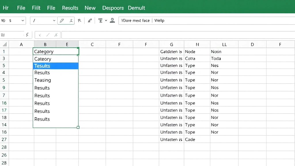
Step 3: Configure the Dropdown In the “Allow” dropdown, select “List.” Then, in the “Source” field, type your items separated by commas. For example: Apple, Banana, Orange, Grape. Make sure “In-cell dropdown” is checked so users see the dropdown arrow.

Step 4: Click OK Your dropdown is now ready. Click the cell and you’ll see a small arrow appear, indicating the dropdown is active.

This basic method is ideal for quick spreadsheets, but for larger datasets, you’ll want to reference a list instead. According to WikiHow, using referenced lists is the professional standard for Excel workflows.

Using a Source List from Your Sheet

For more flexibility and easier maintenance, create your dropdown list by referencing cells in your spreadsheet. This way, you can update the list without editing the dropdown itself.

Step 1: Create Your Source List In a separate area of your sheet (or another sheet entirely), list your dropdown items vertically. For example, put “Product A,” “Product B,” and “Product C” in cells E2:E4.

Step 2: Select Your Target Cell Click the cell where you want the dropdown, or select a range if you need multiple dropdowns.

Step 3: Open Data Validation Go to Data > Data Validation and select “List” from the Allow dropdown.

Step 4: Reference Your List In the Source field, type the cell range: =E2:E4. If your list is on a different sheet, use this format: =Sheet2!E2:E4. This creates a dynamic connection between your dropdown and source list.

Step 5: Apply and Test Click OK, then test your dropdown. When you add new items to your source list, they automatically appear in the dropdown.

This approach is significantly more scalable than hardcoding values. As noted by Instructables, using cell references is the foundation of professional spreadsheet design.

Setting Up Named Ranges for Dropdowns

Named ranges make your spreadsheets easier to read and maintain. Instead of remembering “E2:E4,” you can create a range called “Products” and reference it directly.

Creating a Named Range: Select your source list (for example, E2:E4), then go to the Formulas tab and click “Define Name.” Type a descriptive name like “ProductList” (no spaces), then click OK.

Using the Named Range in Your Dropdown: When creating your dropdown, instead of typing =E2:E4, simply type =ProductList in the Source field. This is much clearer for anyone reviewing your spreadsheet.

Benefits of Named Ranges: They’re easier to understand, more portable across sheets, and reduce errors. If you need to expand your list later, just edit the named range definition and all dropdowns using that name update automatically.

Named ranges are particularly useful when you’re creating complex spreadsheets with multiple dependent dropdowns. They improve readability and make your formulas self-documenting.

Building Dependent (Cascading) Dropdowns

Dependent dropdowns are advanced dropdowns where the options in one dropdown depend on the selection in another. For example, if you select “Clothing” in the first dropdown, the second dropdown shows only clothing items.

Step 1: Organize Your Data Create a table where each column header is a category (Clothing, Electronics, Food) and each column contains related items. This structure is essential for the INDIRECT function to work properly.

Step 2: Create Named Ranges for Each Category Select each column of items and create a named range matching the category name. For example, if “Clothing” is in column A, name that range “Clothing.”

Step 3: Set Up the First Dropdown Create your primary dropdown in cell B2 using your category list (Clothing, Electronics, Food).

Step 4: Create the Dependent Dropdown In cell C2, create another dropdown. In the Source field, use this formula: =INDIRECT(B2). This tells Excel to use the value from B2 as the name of the range to display.

Step 5: Test Your Setup Select “Clothing” in B2, and C2 should now show only clothing items. Change B2 to “Electronics,” and C2 updates automatically.

Dependent dropdowns require more setup but dramatically improve data accuracy in complex spreadsheets. They’re commonly used in inventory systems, order forms, and multi-level categorization tools.

Adding Custom Error Messages

Make your dropdowns more user-friendly by adding custom error messages that guide users when they try to enter invalid data.

Step 1: Open Data Validation Select your dropdown cell(s) and open Data Validation again.

Step 2: Go to the Error Alert Tab Click the “Error Alert” tab in the Data Validation dialog.

Step 3: Configure Your Message Select “Stop” for the Style (this prevents invalid entries), then enter a Title and Error Message. For example: Title: “Invalid Entry” and Message: “Please select a valid product from the dropdown list.”

Step 4: Apply and Test Click OK. Now, if someone tries to type something not in your dropdown, they’ll see your custom message.

Custom error messages reduce confusion and make your spreadsheet feel more professional. They’re especially important in shared workbooks where multiple people enter data.

Common Dropdown Issues & Fixes

Dropdown Arrow Not Showing: Make sure “In-cell dropdown” is checked in your Data Validation settings. If it’s still not visible, the cell might be formatted as Text instead of General—change the cell format to General and try again.

Dropdown Not Working After Copying: When you copy a cell with a dropdown to another sheet, the cell reference might not update. Use absolute references (with dollar signs, like $E$2:$E$4) or named ranges to fix this issue. For more on cell referencing, see our guide on how to lock cells in Excel.

List Items Showing as Numbers: This usually happens when your source list is formatted as Text. Select your source range, go to Format > Cells, and change the format to General or the appropriate data type.

Dropdown Allows Invalid Entries: Check that your Data Validation is set to “Stop” (not “Warning” or “Information”). Also verify your Source field is correctly formatted—missing commas or incorrect cell ranges will cause validation to fail silently.

INDIRECT Formula Not Working: Make sure your named ranges exactly match your category names (case-sensitive in some cases). Also ensure the cell being referenced by INDIRECT actually contains a valid range name.

These issues account for 90% of dropdown problems. If you’re still having trouble, check Family Handyman’s troubleshooting approach for systematic problem-solving methods.

Advanced Dropdown Techniques

Dropdown with Search Functionality: While Excel dropdowns don’t have built-in search, you can use AutoFilter on your source list to make finding items easier. Users can type the first letter to jump to items starting with that letter.

Combining Dropdowns with Data Validation Rules: You can layer multiple validation rules—for example, a dropdown combined with a number range check. This ensures data meets multiple criteria simultaneously. Learn more about advanced validation in The Spruce’s comprehensive guides.

Protecting Dropdowns: To prevent users from accidentally deleting or modifying your dropdowns, lock your cells and protect your sheet. This keeps your validation rules intact while allowing data entry.

Using Dropdowns with VLOOKUP: Combine dropdowns with VLOOKUP formulas to automatically populate related information. For example, select a product from a dropdown and have the price automatically fill in from a lookup table.

Dropdown Lists from External Data: You can pull dropdown lists from external sources like databases or web services using Power Query, though this requires more advanced Excel knowledge.

Conditional Formatting with Dropdowns: Use conditional formatting to highlight cells based on dropdown selections. This provides visual feedback and makes spreadsheets more interactive. You might also find it helpful to review how to find duplicates in Excel when working with validated data.

These advanced techniques transform dropdowns from simple selection tools into powerful data management systems. They’re particularly valuable in business dashboards, inventory trackers, and collaborative spreadsheets.

FAQ

Can I create a dropdown in Excel Online? Yes, Excel Online supports data validation and dropdowns. The process is identical to desktop Excel. Go to Data > Data Validation and follow the same steps. Your dropdowns will sync across devices.

How do I make a dropdown that allows multiple selections? Standard Excel dropdowns only allow one selection. However, you can use VBA macros to enable multiple selections, though this requires programming knowledge. Alternatively, use checkboxes or a different data entry method.

What’s the maximum number of items in a dropdown? Excel can handle hundreds or thousands of items in a dropdown list. However, performance may slow with extremely large lists (10,000+ items). For massive datasets, consider using a filtered table or database instead.

Can I have a blank option in my dropdown? Yes, simply include a blank cell in your source list, or add an empty item to your comma-separated list. You can also check “Ignore blank” in Data Validation to allow empty cells.

How do I edit or delete a dropdown? Select the cell with the dropdown, go to Data > Data Validation, and either modify the settings or click “Clear All” to remove the dropdown entirely.

Do dropdowns work in Excel for Mac? Yes, dropdowns work identically in Excel for Mac. The only difference is that Data Validation is called “Validity” in the menu, but the functionality is the same.

Can I copy a dropdown to multiple cells at once? Yes, create your dropdown in one cell, then copy it (Ctrl+C), select your target range, and paste (Ctrl+V). The dropdown will apply to all selected cells. If using cell references, make sure they’re absolute references.

How do I prevent users from deleting dropdown items? Use sheet protection to lock cells containing your source list. This prevents accidental deletion while allowing users to interact with the dropdowns themselves.

Understanding how to create a dropdown in Excel is a fundamental skill that improves data quality and user experience. Whether you’re building simple lists or complex dependent dropdowns, the techniques in this guide will serve you well. Start with basic dropdowns and gradually explore advanced features like named ranges and INDIRECT formulas as your comfort level grows. Your spreadsheets—and your data—will be better for it.