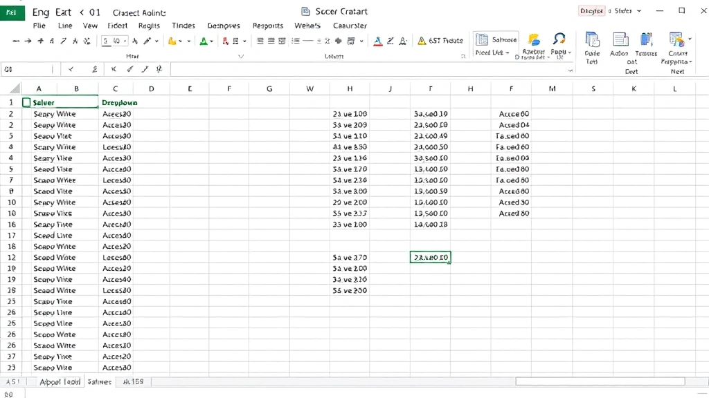
How to Create a Drop Down List in Excel: Easy & Complete Guide

Drop down lists in Excel save time and reduce errors by letting users select from predefined options instead of typing. Whether you’re building a budget tracker, inventory system, or survey form, mastering data validation is essential. This guide walks you through creating, customizing, and managing drop down lists like a pro.
Quick Answer: To create a drop down list in Excel, select your target cells, go to the Data tab, click Data Validation, choose “List” as the Allow option, enter your list items (comma-separated or cell range), and click OK. You can customize error messages, add dependent lists, and even use formulas for dynamic options. The entire process takes just 2-3 minutes once you understand the basics.
Tools & Materials
- Microsoft Excel (2016 or later, or Excel Online)
- A list of items for your drop down (typed or in cells)
- Basic keyboard and mouse skills
- Optional: Named ranges for advanced functionality
- Optional: INDIRECT or INDEX/MATCH formulas for dependent lists
The Basics: Creating Your First Drop Down List
Learning how to create a drop down list in Excel starts with understanding the Data Validation feature. This powerful tool restricts cell entries to specific values, ensuring data consistency across your spreadsheet. When properly implemented, drop down lists make spreadsheets more user-friendly and professional.
Step-by-step process: First, open your Excel file and select the cell or range where you want the drop down to appear. Navigate to the Data tab in the ribbon, then click Data Validation (in older versions, this might be labeled Validity). In the dialog box that opens, change the “Allow” dropdown from “All” to “List”. Now you’re ready to enter your items.
The beauty of how to create a drop down list in Excel is its flexibility. You can type items directly, separated by commas, or reference a range of cells containing your list. For example, typing “Red, Blue, Green” creates a three-option drop down. Alternatively, if your items live in cells A1:A5, you can reference that range instead. This approach is particularly useful when your list changes frequently.
After entering your items, click OK. Your selected cell now displays a small dropdown arrow when clicked, revealing all available options. This visual indicator immediately tells users the cell contains predefined choices.

Three Methods to Create Drop Down Lists
Excel offers multiple approaches to how to create a drop down list in Excel, each suited to different scenarios. Understanding these methods helps you choose the most efficient approach for your specific needs.
Method 1: Direct Text Entry
This is the quickest method for small, static lists. In the Data Validation dialog, select “List” and type your items directly into the Source field, separating each item with a comma and space. For instance, “Yes, No, Maybe” creates a three-option drop down. This method works best for lists with fewer than 10 items that rarely change.
Method 2: Cell Range Reference
For larger or frequently updated lists, reference a cell range instead. If your items are stored in cells D1:D20, enter “=$D$1:$D$20” in the Source field (use absolute references with dollar signs to prevent the range from shifting when copied). This method ensures your drop down always reflects current values. It’s particularly valuable for maintaining a single source of truth for your data.
Method 3: Named Range
Named ranges provide the most professional approach for complex spreadsheets. First, select your list items and assign them a name through the Name Manager (Formulas tab > Define Name). Then, in Data Validation, simply enter the range name as your source. This method offers flexibility and makes your formulas more readable and maintainable.
Customizing Your Drop Down List
Once you understand the basic how to create a drop down list in Excel, customization transforms it into a powerful user experience tool. The Data Validation dialog contains several tabs offering extensive customization options.
Input Message tab: Add a helpful prompt that appears when users click your drop down cell. For example, “Select your department from the list below” guides users and prevents confusion. This message displays as a small tooltip, improving usability without cluttering your spreadsheet.
Error Alert tab: Control what happens when someone tries to enter invalid data. Choose between three alert styles: Stop (prevents invalid entries), Warning (allows but discourages invalid entries), and Information (simply notifies). Customize the error title and message to match your spreadsheet’s purpose. A clear error message like “Please select from the provided list” helps users correct mistakes quickly.
Show dropdown arrow: Ensure the “Show dropdown arrow” checkbox is checked so users can easily identify which cells contain drop downs. This visual cue significantly improves spreadsheet navigation and reduces user errors.

Building Dependent Drop Down Lists
Advanced users can create dependent drop downs, where one list’s options depend on another list’s selection. This sophisticated technique is invaluable for hierarchical data. For example, selecting “North America” in one drop down might display only “USA, Canada, Mexico” in a dependent drop down.
To build dependent drop downs, you’ll need to create separate named ranges for each category. First, organize your data with categories in column A and subcategories in columns B, C, and D. Select each subcategory range and assign it a name matching its category (for instance, name the USA cities range “USA”).
In your dependent drop down cell, use an INDIRECT formula as the source: “=INDIRECT(A1)” where A1 contains your first drop down. This formula dynamically references the named range corresponding to the selected category. While this requires more setup, the result is an elegant, professional data entry system.
Adding Data Validation Rules
Data validation rules strengthen how to create a drop down list in Excel by preventing invalid entries. Beyond basic lists, you can validate numeric ranges, dates, text length, and custom formulas.
Numeric validation: Select “Whole Number” or “Decimal” to restrict entries to specific ranges. For instance, allowing only values between 1 and 100 ensures data consistency in scoring systems. This prevents users from accidentally entering invalid numbers.
Date validation: Choose “Date” to restrict entries to specific date ranges. This is particularly useful for project timelines, appointment scheduling, or deadline tracking. You can set minimum and maximum dates, ensuring entries fall within acceptable parameters.
Custom formulas: For complex validation needs, create custom formulas using the “Custom” option. For example, “=AND(A1>0, A1<100)" validates that cell A1 contains a value between 0 and 100. This advanced technique enables sophisticated business logic within your spreadsheet.
Common Issues & Solutions
Even experienced users encounter challenges when working with drop downs. Understanding common problems helps you troubleshoot quickly and maintain spreadsheet integrity.
Drop down arrow not showing: Ensure the “Show dropdown arrow” option is checked in Data Validation settings. If it’s checked but still not visible, try clicking the cell again. Sometimes Excel requires a refresh to display the arrow properly.
List items not appearing: Verify that your source range contains data and uses correct syntax. If using a named range, confirm it’s spelled correctly and actually contains values. Empty cells in your source range won’t appear in the drop down.
Drop down not copying correctly: When copying cells with drop downs to other locations, use Paste Special and select “Validation” to ensure drop down rules transfer properly. Regular copy-paste might not include validation settings.
Circular reference errors: If using formulas in your drop down source, ensure they don’t reference the cell containing the drop down itself. This creates a circular reference that Excel cannot resolve.
Advanced Techniques
Master how to create a drop down list in Excel by exploring advanced techniques that power professional spreadsheets. These methods combine multiple Excel features for sophisticated data management.
Multi-column drop downs: While Excel’s native drop downs display single columns, you can create the illusion of multi-column lists using helper columns and VLOOKUP formulas. This technique displays additional information when users select an option, enriching the user experience.
Searchable drop downs: For large lists, implement searchable functionality using AutoFilter on your data source. Users can type to filter options quickly, dramatically improving usability for lists exceeding 20 items.
Dynamic lists with UNIQUE function: In Excel 365, use the UNIQUE function to create drop downs from dynamic ranges that automatically exclude duplicates. This ensures your drop down always displays clean, unique values.
Conditional formatting with drop downs: Combine drop downs with conditional formatting to highlight cells based on selected values. For instance, selecting “High Priority” automatically highlights the cell in red, creating visual organization.
According to WikiHow, mastering data validation features significantly improves spreadsheet efficiency. For additional insights on Excel functionality, Family Handyman’s practical approach to tutorials demonstrates how proper setup prevents future problems. Instructables also offers community-verified methods for complex Excel techniques.
If you’re managing complex spreadsheets, you might also benefit from learning how to freeze a row in Excel, which helps maintain header visibility while scrolling through data-heavy sheets. This complements drop down lists perfectly when organizing large datasets.
For those working across different Office applications, understanding how to double space in Word helps maintain consistent document formatting standards across your workflow.

FAQ
Can I create drop downs in Excel Online?
Yes, Excel Online supports data validation and drop down lists. The process is nearly identical to desktop Excel, though some advanced features like INDIRECT formulas may have limitations. Access Data Validation through the Data tab in the ribbon.
How do I delete a drop down list?
Select the cell containing the drop down, go to Data > Data Validation, and click “Clear All”. This removes all validation rules from the selected cell while preserving any existing data.
Can drop down lists contain formulas?
Yes, your source range can contain formulas that generate list items dynamically. However, the drop down itself displays only the formula results, not the formulas themselves.
What’s the maximum number of items in a drop down list?
Excel supports up to 32,767 characters in a single cell validation source. For practical purposes, most drop downs contain between 5 and 100 items for optimal usability.
How do I make drop downs case-sensitive?
Excel’s standard drop downs are not case-sensitive. To enforce case sensitivity, use custom validation formulas with the EXACT function to compare entries against your list.
Can I create drop downs in Excel for Mac?
Absolutely. Excel for Mac includes the same Data Validation features as Windows versions. The process is identical, though menu locations might vary slightly depending on your Mac Excel version.
How do I copy drop down lists to multiple cells efficiently?
Create your drop down in one cell, copy it, select your target range, then use Paste Special (Ctrl+Shift+V) and select “Validation” to paste only the drop down rules without affecting existing cell content.
Can drop downs work with conditional logic?
Yes, combine drop downs with IF formulas to create intelligent lists that change based on other cell values. This creates responsive spreadsheets that adapt to user input automatically.


