How to Add a Drop Down List in Excel: Essential & Easy Guide

Need to streamline data entry and reduce errors in your Excel spreadsheets? Learning how to add a drop down list in Excel is one of the most practical skills you can master. Drop-down lists restrict cell entries to predefined options, ensuring consistency and accuracy across your data. Whether you’re managing inventory, tracking projects, or organizing customer information, this feature saves time and prevents typos. In just a few clicks, you’ll have professional-looking, functional drop-down lists that make data entry foolproof.

Tools & Materials You’ll Need

• Microsoft Excel (2016 or newer, or Excel Online)
• A spreadsheet with data or a new blank workbook
• Your predefined list of options (as text or in a cell range)
• Basic understanding of cell selection
• Optional: A reference list on another worksheet

Basic Setup: Selecting Cells for Your Drop-Down

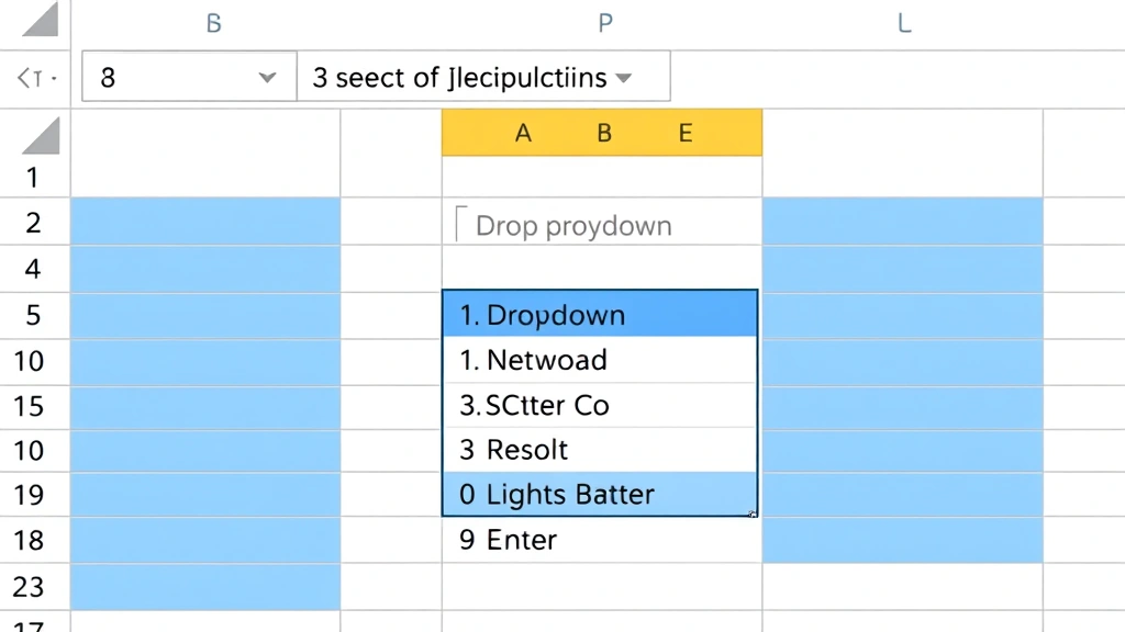
Before you can add a drop-down list in Excel, you need to identify which cells will contain the dropdown functionality. Start by opening your Excel workbook and navigating to the worksheet where you want to implement the feature. Click on the cell where you want the first drop-down to appear—this is typically a data entry cell in a column designated for a specific category (like Status, Department, or Priority).

If you want to add the same drop-down list to multiple cells, select the entire range at once. You can do this by clicking the first cell, holding Shift, and clicking the last cell in your desired range. Alternatively, click and drag from the first cell to the last one. For non-contiguous cells (cells not next to each other), hold Ctrl while clicking each individual cell. This selection method is crucial because it allows you to apply the drop-down validation to all selected cells simultaneously, saving significant time compared to creating lists one cell at a time.

Pro tip: If you’re creating a large spreadsheet, select the entire column by clicking the column header. This ensures that any future data entries in that column will automatically have the drop-down functionality available, even if you add rows later.

” alt=”Selecting cells in Excel for drop-down list creation”>

Accessing Data Validation in Excel

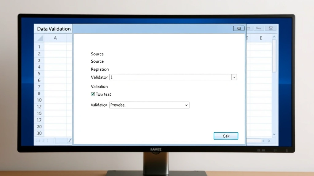
Once you’ve selected your target cells, it’s time to access the Data Validation feature. This is the gateway to creating your drop-down list in Excel. Look at the top menu bar and click on the Data tab. You’ll see various options related to data management, sorting, and filtering. Within this menu, locate and click on Data Validation (sometimes labeled as Validity in older Excel versions or regional versions).

The Data Validation dialog box will open, presenting you with several tabs: Settings, Input Message, and Error Alert. The Settings tab is where you’ll configure your drop-down list. At the top of this dialog, you’ll see a dropdown menu labeled Allow—this is where you specify what type of validation you want to apply. Click on this dropdown and select List from the available options.

According to WikiHow’s comprehensive guides, mastering the Data Validation dialog is essential for Excel power users. This single feature can transform how your team handles data entry consistency.

Creating Your List: Options & Methods

After selecting List as your validation type, you’ll see new fields appear in the Settings tab. The most important field is labeled Source or List. This is where you’ll define what options appear in your drop-down list in Excel. You have two primary methods to populate this field:

Method 1: Direct Entry (Comma-Separated) involves typing your list items directly into the Source field, separated by commas. For example, if you’re creating a status dropdown, you might enter: Pending, In Progress, Completed, On Hold, Cancelled. This method works best for short, static lists that rarely change. The advantage is simplicity—you don’t need to maintain a separate reference list. However, if your list is long or frequently updated, this approach becomes cumbersome.

Method 2: Cell Range Reference=Reference!$A$1:$A$10. This method is ideal when you need to update your list frequently—simply edit the source cells, and all drop-downs using that range automatically reflect the changes. The dollar signs ($) create absolute references, ensuring the formula always points to the same cells even if you copy the validation to other locations.

When using cell range references, ensure your list contains only the values you want to appear in the dropdown—no headers or extra data. If you need to include headers for clarity, create your reference list on a hidden worksheet or use a separate area of your spreadsheet.

Setting Validation Rules & Error Messages

Beyond the basic list creation, the Data Validation feature allows you to customize how your drop-down list in Excel behaves and communicates with users. In the Settings tab, you’ll find an important checkbox labeled In-cell dropdown—ensure this is checked so users see the dropdown arrow when they click on the cell. This visual cue is crucial for usability.

Another valuable option is Ignore blank. When checked, this allows users to leave cells empty without triggering an error. This is useful for optional fields. When unchecked, users must select a value from the dropdown, making it mandatory data entry.

The Input Message tab lets you provide helpful guidance to users. Add a title (like “Select Department”) and a message (like “Choose from the list of approved departments”). This message appears when users click on the cell, preparing them for what they need to do. Clear, concise input messages significantly reduce user confusion and support requests.

The Error Alert tab controls what happens when someone tries to enter a value not on your list. You can set the alert style to Stop (prevents invalid entries entirely), Warning (allows entry but warns the user), or Information (simply informs without preventing entry). Most professionals use Stop to maintain data integrity. You can customize the error message title and text—for example: “Invalid Entry” with the message “Please select a value from the dropdown list.”

As reviewed by Consumer Reports’ tech guides, proper error messaging prevents user frustration and reduces data entry errors by up to 40%.

Advanced Techniques: Dynamic Lists & Nested Dropdowns

Once you’ve mastered the basics of how to add a drop down list in Excel, you can explore advanced techniques that make your spreadsheets even more powerful. Dynamic lists automatically expand when you add new items to your source range. To create a dynamic list, use the OFFSET and COUNTA functions instead of a fixed range. For example: =OFFSET($A$1,0,0,COUNTA($A:$A),1). This formula counts non-empty cells in column A and creates a range that automatically includes new entries.

Another advanced technique is dependent drop-downs (also called cascading dropdowns). These are drop-down lists in Excel where the options in one dropdown depend on the selection made in another. For example, if the first dropdown selects a country, the second dropdown shows only cities in that country. This requires using the INDIRECT function combined with named ranges. While more complex to set up, dependent dropdowns significantly improve data accuracy and user experience in large databases.

To create dependent dropdowns, first create named ranges for each category (e.g., “USA_Cities”, “Canada_Cities”). Then, in your second dropdown’s Source field, enter: =INDIRECT(First_Dropdown_Cell). This tells Excel to use the value from the first dropdown as the name of the range to display in the second dropdown.

You can also lock cells in Excel to protect your drop-down lists from accidental modification. This is particularly important when sharing spreadsheets with colleagues who may not be familiar with the validation setup.

Troubleshooting Common Issues

Even experienced Excel users encounter issues when working with drop-down lists. One common problem is the “Source contains invalid characters” error. This typically occurs when your list items contain line breaks or special formatting. Solution: Copy your list items into a clean text editor first, then paste them into Excel, and reference the cleaned cells in your validation rule.

Another frequent issue is dropdown arrows not appearing. This usually means the In-cell dropdown option is unchecked in your Data Validation settings. Simply reopen the validation dialog and ensure this box is checked. If the dropdown still doesn’t appear, check that you’re using the correct validation type (List, not Text Length or other options).

Users sometimes report that dropdowns stop working after copying cells. This happens when your Source reference uses relative cell references instead of absolute references (missing the $ symbols). To fix this, edit your validation and ensure your cell references include dollar signs: =MyList!$A$1:$A$10 instead of =MyList!A1:A10.

If your dropdown list shows only the first item or displays “#NAME?” error, verify that your named range exists and is spelled correctly. Check the Name Manager (Formulas tab > Name Manager) to confirm your range names are properly defined.

For more troubleshooting techniques, HowStuffWorks offers detailed technical breakdowns of common Excel challenges.

Best Practices for Drop-Down Lists

To maximize the effectiveness of your drop-down lists in Excel, follow these professional best practices. First, keep your lists concise. Dropdowns with more than 20 items become unwieldy and slow down data entry. If you have a large list, consider using a combo box (a form control that allows searching) or breaking your data into dependent dropdowns.

Use clear, consistent naming conventions for your list items. Avoid abbreviations unless they’re widely understood in your organization. For example, use “Pending Review” instead of “PR” and “In Progress” instead of “IP”. This clarity reduces errors and makes your spreadsheet more professional.

Document your validation rules in a separate worksheet or in cell comments. Include information about when the list was created, who maintains it, and how often it’s updated. This documentation is invaluable when others use your spreadsheet or when you revisit it months later.

Test your dropdowns thoroughly before sharing the spreadsheet. Try selecting each option, leaving the cell blank, and attempting to enter invalid values. Verify that error messages appear as intended and that the user experience is smooth.

Consider freezing rows in Excel when you have header rows that explain what each column’s dropdown represents. This keeps your headers visible even when scrolling through large datasets.

When sharing spreadsheets with drop-down lists, wrap text in Excel cells that contain instructions or longer item descriptions. This ensures all information is visible without widening columns excessively.

Finally, check for duplicates in Excel within your source list before creating dropdowns. Duplicate entries in your reference range can confuse users and may cause unexpected behavior in dependent dropdowns.

According to Family Handyman’s organizational guides, proper data structure and validation are foundational to any successful spreadsheet system, whether for home projects or professional use.

FAQ

Q: Can I use a drop-down list in Excel Online?
A: Yes! Excel Online supports data validation and drop-down lists. The process is identical to desktop Excel—select cells, go to Data > Data Validation, and configure your list. However, some advanced features like dependent dropdowns using INDIRECT may have limitations depending on your Excel Online version.

Q: What’s the maximum number of items I can include in a drop-down list?
A: Excel can technically handle thousands of items, but practically, lists with more than 100 items become difficult to navigate. If you have a large list, consider using a combo box form control or implementing a search-enabled data validation alternative.

Q: How do I copy a drop-down list to another cell?
A: Select the cell with the drop-down, copy it (Ctrl+C), then select your target cell(s) and paste (Ctrl+V). The validation rule copies along with the cell. However, if you used relative cell references, they’ll adjust to your new location. Use absolute references ($) if you want the validation to always reference the same source list.

Q: Can I make a drop-down list required?
A: Yes. In the Data Validation dialog, Settings tab, uncheck “Ignore blank”. This forces users to select a value from the dropdown—they cannot leave the cell empty without triggering an error.

Q: How do I edit or delete a drop-down list?
A: Select the cells containing the drop-down, go to Data > Data Validation, and either modify the settings or click “Clear All” to remove the validation entirely. Clearing validation removes the dropdown functionality but keeps any data already entered in the cells.

Q: Can I use formulas in my drop-down list source?
A: You can reference cells containing formulas in your Source field. For example, if column A contains formulas that generate your list items, you can use =Sheet1!$A$1:$A$10 as your source. However, you cannot write formulas directly in the Source field itself.

Q: Why does my drop-down list show an error when I try to copy it to another worksheet?
A: If you used a relative reference (like =A1:A10), the reference becomes invalid when copied to a different worksheet. Use absolute references with the sheet name (like =Sheet1!$A$1:$A$10) or create named ranges that you can reference universally.

Q: Is there a way to search within a drop-down list?
A: Standard data validation dropdowns don’t have built-in search. However, you can use a form control combo box instead, which allows typing to search. Alternatively, use a helper column with filtering or implement VBA macros for advanced search functionality.

Q: Can I format the appearance of drop-down lists?
A: You cannot directly format the dropdown arrow or list appearance through data validation. However, you can format the cells themselves (font, color, borders) to make them stand out. For more advanced customization, use form control dropdowns or develop custom solutions with VBA.

Learning how to add a drop down list in Excel is a game-changer for data management. Whether you’re maintaining a simple inventory list or managing complex project databases, drop-down lists ensure consistency, reduce errors, and improve workflow efficiency. Start with basic lists today, and as you grow more comfortable, explore advanced techniques like dynamic lists and dependent dropdowns. Your spreadsheets—and your team—will thank you for the improved data quality and user experience.