Excel How to Check Duplicate: Simple & Essential Guide

Quick Answer: Use Excel’s Conditional Formatting feature to highlight duplicates instantly, or apply the Remove Duplicates tool to delete them. For more control, use COUNTIF formulas to identify which rows contain duplicate values. The method you choose depends on whether you want to flag duplicates for review or eliminate them permanently.

Tools & Materials You’ll Need

• Microsoft Excel (2016 or newer) or Google Sheets
• Your dataset with potential duplicate entries
• A backup copy of your original file (recommended)
• Basic understanding of cell references and ranges
• Optional: COUNTIF, MATCH, or INDEX formulas for advanced detection

Why Checking for Duplicates Matters

Duplicate entries are one of the most common data quality issues in spreadsheets. When you fail to check for duplicates in Excel, you risk inflating metrics, double-counting revenue, or sending duplicate communications to customers. A single duplicate entry might seem harmless, but in large datasets, duplicates compound errors exponentially.

According to Consumer Reports, data accuracy is critical for business decisions. Knowing how to check duplicate values ensures your analysis reflects reality, not corrupted data. Whether you’re preparing reports for executives, reconciling accounts, or cleaning imported data, mastering duplicate detection saves hours of manual review.

Key benefits of checking for duplicates:

• Improves data accuracy and reporting reliability
• Prevents double-counting in financial or inventory systems
• Reduces wasted effort on redundant entries
• Ensures compliance with data governance standards
• Streamlines workflows and decision-making

Method 1: Highlight Duplicates with Conditional Formatting

Conditional Formatting is the fastest way to visually identify duplicates without altering your data. This method lets you review flagged entries before taking action, making it ideal for critical datasets where you need to verify duplicates manually.

Step-by-step process to check duplicate entries using Conditional Formatting:

1. Select your data range: Click the first cell in your column and drag to select all data. Alternatively, click the column header to select the entire column.
2. Open Conditional Formatting menu: Go to the Home tab, then click Conditional Formatting (usually in the Styles group).
3. Choose “Highlight Cell Rules”: Hover over the option and select Duplicate Values.
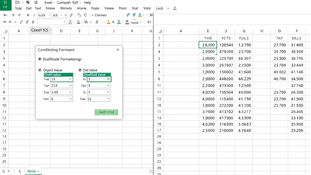
4. Set formatting options: A dialog box appears. Leave the default setting as “Duplicate” and choose your preferred highlight color (red, yellow, or light red are common choices).
5. Click OK: Excel instantly highlights all duplicate values in your selected range with the chosen color.

This method is particularly useful when you want to preserve all data while visually flagging duplicates for investigation. You can then manually review each highlighted entry to determine whether it’s a true duplicate or a legitimate repeat entry (like multiple orders from the same customer).

Pro tip: To remove the conditional formatting later, select your range, go to Conditional Formatting > Clear Rules > Clear Rules from Selected Cells.

Method 2: Use the Remove Duplicates Tool

When you’re confident about your data and ready to eliminate duplicates permanently, Excel’s built-in Remove Duplicates tool is the most efficient solution. This feature compares rows and deletes exact matches, keeping only the first occurrence of each unique entry.

How to use the Remove Duplicates tool to check and eliminate duplicates:

1. Create a backup: Always save a copy of your original file before removing duplicates permanently.
2. Select your data: Highlight the entire data range, including headers if present.
3. Access the Data tab: Click the Data menu at the top of the ribbon.
4. Click “Remove Duplicates”: This option is usually in the Data Tools group. A dialog box opens showing all columns in your selection.
5. Choose columns to compare: By default, all columns are selected. Uncheck any columns you want to exclude from duplicate checking. For example, if you only want to check for duplicate names (not duplicate addresses), uncheck the address column.
6. Confirm headers: Check the “My data has headers” option if your first row contains column titles.
7. Click OK: Excel removes all duplicate rows and displays a confirmation message showing how many duplicates were deleted.

This method is decisive and permanent, so ensure you understand your data before applying it. The tool keeps the first occurrence of each duplicate set and removes subsequent matches. If you need more nuanced control, consider using formulas instead.

Method 3: Identify Duplicates with COUNTIF Formula

For advanced users who need precise control, the COUNTIF formula is the gold standard for checking duplicates in Excel. This formula counts how many times each value appears in your range, allowing you to flag entries that appear more than once.

Using COUNTIF to check duplicate values:

1. Create a helper column: Insert a new column next to your data (e.g., column B if your data is in column A).
2. Enter the COUNTIF formula: In the first cell of your helper column, type: =COUNTIF($A$2:$A$100,A2)
3. Adjust the range: Replace A2:A100 with your actual data range. The dollar signs ($) create absolute references so the range doesn’t change when you copy the formula down.
4. Copy the formula: Select the cell with your formula and drag down to apply it to all rows in your dataset.
5. Interpret results: Any cell showing “1” appears only once (unique). Any cell showing “2” or higher indicates a duplicate. For example, a result of “3” means that entry appears three times in your data.

This approach gives you visibility into exactly how many times each entry repeats. You can then sort by the helper column to group all duplicates together, making manual review and decision-making easier. As noted by WikiHow, formulas provide flexibility that automated tools sometimes lack.

Example formula breakdown:

• COUNTIF = the function that counts cells matching a criterion
• $A$2:$A$100 = the absolute range to search (won’t change when copied)
• A2 = the criterion (the value in the current row to match)

Method 4: Advanced Duplicate Detection Techniques

When dealing with complex datasets or multiple columns, advanced techniques provide more sophisticated duplicate detection. These methods are particularly useful when you need to identify duplicates based on combinations of columns rather than single values.

Using MATCH and INDEX for duplicate detection:

The MATCH function finds the position of a value within a range, helping you identify whether the current row is the first occurrence of a duplicate set. Combine it with IF to create a formula like: =IF(MATCH(A2,$A$2:$A$100,0)=ROW()-1,"First","Duplicate")

This formula labels the first occurrence of each value as “First” and subsequent occurrences as “Duplicate.” It’s more nuanced than simple counting and helps you preserve the original entry while flagging copies.

Checking duplicates across multiple columns:

If your data spans multiple columns and you want to find rows that are completely identical, concatenate columns in a helper column first. Use a formula like: =A2&B2&C2 to combine values, then apply COUNTIF to this concatenated result. This method identifies exact row duplicates across multiple fields.

For users working with large datasets, these advanced techniques integrate seamlessly with Excel’s filtering and sorting capabilities, enabling efficient data management without external tools.

Method 5: Filter and Sort to Find Duplicates

Sometimes the simplest approach is the most effective. Sorting and filtering your data manually helps you visually identify duplicates without complex formulas or special tools. This method works best for smaller datasets where you have time for careful review.

Steps to filter and sort for duplicate detection:

1. Select your data: Highlight the range you want to analyze.
2. Apply AutoFilter: Go to Data > Filter > AutoFilter. Dropdown arrows appear in your header row.
3. Sort by your key column: Click the dropdown arrow in the column you suspect contains duplicates and select Sort A to Z (or Z to A). Identical values now group together.
4. Visual scan: Scroll through your sorted data and manually identify adjacent rows with identical values.
5. Use additional filters: Click column dropdowns to filter for specific values, narrowing your focus to potential duplicates.

This method is transparent and requires no formulas, making it accessible to all Excel users. However, it’s time-consuming for large datasets. Combine it with the alphabetize in Excel technique to organize data logically before review.

Best Practices for Managing Duplicates

Knowing how to check duplicate entries is only half the battle. Implementing best practices ensures your data remains clean and duplicate-free going forward.

Prevention strategies:

• Use data validation: As explained in our guide on how to create a dropdown in Excel, dropdowns restrict entry options and reduce manual entry errors that create duplicates.
• Implement unique identifiers: Assign ID numbers or codes to each record. Duplicates become obvious when IDs repeat.
• Establish data entry protocols: Train users to check for existing entries before adding new ones.
• Schedule regular audits: Check for duplicates monthly or quarterly, depending on data volume and turnover.

When removing duplicates, follow these guidelines:

• Always backup first: Save your original file before applying the Remove Duplicates tool.
• Document your process: Record which columns you used for duplicate checking and how many duplicates were removed. This creates an audit trail.
• Review before deleting: Use Conditional Formatting to visually verify duplicates match your expectations before permanent deletion.
• Consider business logic: Not all repeating values are errors. Multiple orders from the same customer are legitimate, not duplicates.

According to Lifehacker, maintaining clean data is an ongoing process, not a one-time fix. Integrate duplicate checking into your regular spreadsheet maintenance routine.

For related data management tasks, explore how to lock a row in Excel to protect header information while working with large datasets, or learn how to subtract in Excel for financial reconciliation tasks that often reveal duplicate entries.

FAQ

Q: Can I check for duplicates in Google Sheets the same way as Excel?
A: Google Sheets has similar tools. Use Format > Conditional Formatting > Custom Formula or the built-in duplicate highlighting feature. The Remove Duplicates function is also available under Data > Data Cleanup > Remove duplicates. The process is nearly identical to Excel.

Q: What’s the difference between “Remove Duplicates” and “Conditional Formatting”?
A: Remove Duplicates permanently deletes duplicate rows from your spreadsheet. Conditional Formatting only highlights duplicates visually without changing your data. Use Conditional Formatting for review and analysis; use Remove Duplicates when you’re ready to clean your data permanently.

Q: Can I check for duplicates based on partial matches (like similar but not identical text)?
A: Excel’s built-in tools look for exact matches only. For fuzzy matching (finding similar entries with minor spelling variations), you’ll need advanced formulas or third-party add-ins. Manually review flagged entries or use specialized data cleaning software for this level of sophistication.

Q: How do I handle duplicates when I want to keep all instances but just identify them?
A: Use Conditional Formatting or the COUNTIF formula method. Both highlight or flag duplicates without deleting them. You can then manually decide which copies to keep based on your business needs.

Q: Will removing duplicates affect my formulas that reference those cells?
A: Yes. If other cells contain formulas referencing deleted rows, those formulas may return errors. Always audit your spreadsheet for dependent formulas before removing duplicates, and consider using named ranges or absolute references to minimize breakage.

Q: What if my dataset has thousands of rows? Which method is fastest?
A: For very large datasets, the Remove Duplicates tool is fastest because it processes all rows at once. The COUNTIF formula method is slower but more transparent. Conditional Formatting can lag on huge datasets, so reserve it for smaller ranges when working with thousands of rows.

Q: Can I undo the Remove Duplicates action?
A: Yes, immediately after removing duplicates, press Ctrl+Z (or Cmd+Z on Mac) to undo. However, if you’ve saved the file, the action is permanent. This is why creating backups before removing duplicates is essential.