How to Freeze Columns in Excel: Easy & Essential Guide

You’re staring at a massive spreadsheet with hundreds of rows and dozens of columns. You scroll right to check a calculation, and suddenly you’ve lost sight of the column headers that tell you what each data point means. Sound familiar? Learning how to freeze columns in Excel solves this exact problem and saves you from the frustration of constant scrolling. Whether you’re managing inventory, tracking sales data, or analyzing financial reports, freezing columns keeps your reference data locked in place while you navigate the rest of your sheet. It’s one of those features that seems hidden until you need it, then you wonder how you ever lived without it.

What Does Freezing Columns Actually Do?

Think of freezing columns like putting a bookmark in a book—except instead of marking your place, you’re locking specific columns in view. When you freeze columns in Excel, those columns stay visible on your screen even when you scroll horizontally to the right. The frozen columns remain anchored to the left side of your spreadsheet, creating an invisible divider between what moves and what stays put.

Here’s the real-world scenario: imagine you have a product inventory sheet with 50 columns. Column A contains product names, Column B has SKU numbers, and Columns C through AX contain sales data for different regions and time periods. If you don’t freeze Column A and B, scrolling right to see California sales data means losing sight of what product you’re actually looking at. Freeze those first two columns, and they hang around no matter how far right you travel. You always know exactly which product row you’re examining.

This feature works differently than just making a column wider or using split panes. Microsoft’s official documentation on freezing panes explains that freezing creates a hard lock on columns, preventing them from scrolling with the rest of your data. It’s permanent until you actively unfreeze them, making it ideal for reference columns you’ll need visible constantly.

How to Freeze a Single Column (Step-by-Step)

Freezing a single column is the most common use case, and it’s simpler than you might think. Here’s the exact process:

1. Click on the column header to the right of the column you want to freeze. This is the critical step that trips people up. If you want Column A frozen, you click on Column B’s header. If you want Columns A and B frozen, you click on Column C. You’re essentially telling Excel: “Everything to the left of where I click stays put.”
2. Navigate to the View tab in the ribbon. At the top of your Excel window, you’ll see tabs like Home, Insert, Page Layout, and View. Click View.
3. Look for the Freeze Panes option. In the View ribbon, you’ll see a button labeled “Freeze Panes” with a small dropdown arrow next to it. Click the dropdown arrow to see your options.
4. Select “Freeze Panes” from the menu. A submenu appears with three choices: Freeze Panes, Freeze First Column, and Freeze First Row. Choose “Freeze Panes.”
5. Verify the freeze line appears. After clicking, you should see a slightly thicker line (usually darker or slightly raised) between the frozen and unfrozen columns. This visual indicator confirms your freeze is active.

Let me walk through a concrete example. Say you’re working with a customer database where Column A contains customer names. You want that column visible at all times. Click on Column B header, go to View → Freeze Panes → Freeze Panes. Done. Now when you scroll right to see email addresses, phone numbers, or purchase history in columns further right, Column A stays locked on the left.

Pro tip: If you mess up and freeze the wrong column, don’t panic. Just go back to View → Freeze Panes and select “Unfreeze Panes.” Then start over with the correct column. There’s no penalty for trying again.

Freezing Multiple Columns at Once

Sometimes a single column isn’t enough reference information. Maybe you need both the customer name AND their account number visible, or perhaps you’re tracking products with both SKU and category data. Freezing multiple columns uses the exact same process, just with a different starting point.

The rule is simple: click on the column header that comes immediately after the last column you want frozen. If you want Columns A, B, and C frozen, click on Column D header. If you want Columns A through E frozen, click on Column F header.

1. Identify your last column to freeze. Let’s say you want Columns A (Product Name), B (SKU), and C (Category) all frozen. Column C is your last frozen column.
2. Click on the next column header (Column D in this example). You’re marking the boundary of your freeze zone.
3. Go to View → Freeze Panes → Freeze Panes. Same menu path as before.
4. Confirm the freeze line appears after Column C. The visual divider should be between Column C and Column D now.

This approach works for up to 26 columns (A through Z) or more in larger spreadsheets. However, here’s real talk: if you’re freezing more than 4-5 columns, you might want to reconsider your spreadsheet layout. Too many frozen columns can make your working area cramped and defeats the purpose of having flexibility in your data view. While Family Handyman focuses on home projects, the principle of “keep your workspace organized” applies to spreadsheets too.

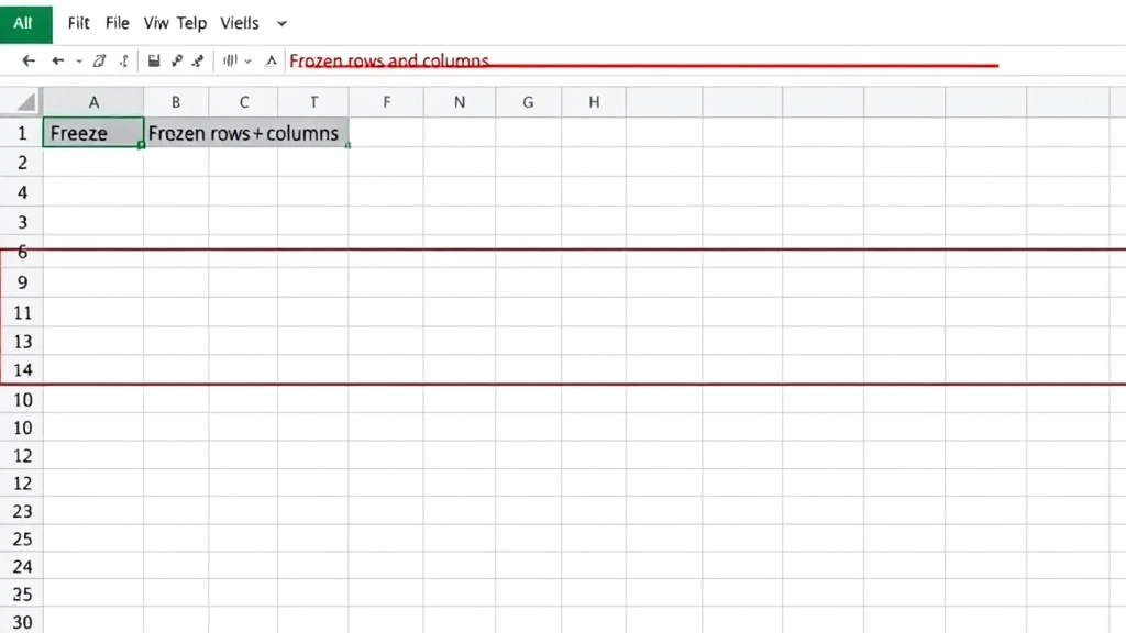
Freezing Both Rows and Columns Together

Here’s where things get powerful. Most spreadsheets have headers in the first row (like “Product Name,” “Quantity,” “Price”) AND reference columns on the left (like product IDs or names). You probably want BOTH frozen simultaneously. This is called freezing panes, and Excel handles it beautifully.

The process is nearly identical to what you’ve already learned, with one key difference:

1. Click on the cell at the intersection of where your freeze lines will be. If you want the first row frozen AND the first three columns frozen, click on cell D2. You’re positioning your cursor at the exact spot where the horizontal and vertical freeze lines will meet.
2. Navigate to View → Freeze Panes → Freeze Panes. Same menu.
3. Observe the freeze lines. You should now see one line below row 1 and another line to the right of Column C. Everything above row 1 and to the left of Column C is now locked in place.

This is particularly useful for large data analysis projects. Imagine a quarterly sales report with months across the top (row 1) and product names down the left (Column A). Freeze at cell B2, and you can scroll through months while always seeing which product you’re analyzing, and you can scroll through products while always seeing which month is active.

Pro tip from the field: This Old House’s approach to systematic organization mirrors how spreadsheet pros organize their data—with clear headers and logical structure. Your frozen zones should reflect your spreadsheet’s natural structure, not fight against it.

How to Unfreeze Columns

Unfreezing is even simpler than freezing. You don’t need to click on a specific column or cell. Excel knows you have a freeze active and gives you the option to remove it.

1. Click on the View tab. Same as before.
2. Click the Freeze Panes dropdown. Look for the Freeze Panes button with the dropdown arrow.
3. Select “Unfreeze Panes.” This option only appears if you currently have a freeze active. Click it, and your freeze is removed instantly.

That’s it. No confirmation dialog, no complexity. Your columns return to normal scrolling behavior immediately. If you accidentally unfroze when you meant to keep it frozen, just re-freeze using the same steps as before.

One thing to note: unfreezing doesn’t affect your data at all. You’re only changing how the spreadsheet displays. All your formulas, values, and formatting stay exactly as they were.

Common Problems & Fixes

– Solution: You’re probably on a sheet with very limited data. Freeze Panes requires at least two columns and two rows to function. If you only have one column or one row of data, Excel disables the freeze option. Add more data or check that you’re on the right worksheet.

– Solution: Unfreeze everything first (View → Freeze Panes → Unfreeze Panes), then take a moment to identify exactly which columns you want frozen. Write it down if needed. Then click on the correct column header and re-freeze. The visual freeze line should be obvious once you know what to look for—it’s a slightly thicker or darker line between columns.

– Solution: You probably clicked on the wrong column header before freezing. Remember: click on the column header that comes AFTER your last frozen column. If you want Column A frozen, click Column B. If you want Columns A and B frozen, click Column C. Unfreeze, then try again with the correct column.

– Solution: You scrolled too far left (which shouldn’t happen) or your frozen columns are hidden. Try pressing Ctrl+Home to jump back to cell A1. If frozen columns are hidden, right-click on the column headers near the freeze line, select “Unhide,” and your frozen columns should reappear. For detailed help with hidden cells, check our guide on how to unhide cells in Excel.

– Solution: Shared workbooks have limitations. Some formatting features, including freezing panes, can behave unpredictably in shared mode. If this is critical, consider having one person maintain the master file with freezes applied, then distribute copies. Alternatively, use Excel’s protection features to lock the freeze in place.

Pro Tips for Power Users

Combine freezing with filtering for maximum control. You can freeze columns AND apply AutoFilter to your data. This means you can freeze reference columns while filtering the remaining columns to show only relevant data. It’s a powerful combo for large datasets. Apply the freeze first, then add your filters.

Use keyboard shortcuts to speed up your workflow. While there’s no direct keyboard shortcut for freezing (it’s menu-based), you can use Alt+W to jump to the View tab quickly, then use arrow keys to navigate to Freeze Panes. It’s faster than clicking once you get the rhythm down.

Freeze strategically based on your audience. If you’re sharing a spreadsheet with others, apply freezes that make sense for how they’ll use the data. A financial analyst needs different frozen columns than a sales manager. Think about your end user’s workflow before freezing.

Document your freeze setup in a separate note or cell.** If you’re creating a complex spreadsheet that others will use, add a comment or note explaining which columns are frozen and why. This prevents confusion and helps new users understand the sheet’s structure immediately.

Remember that frozen columns don’t print by default in the way you might expect. When you print a spreadsheet with frozen columns, Excel prints the entire sheet normally—frozen columns aren’t specially marked. If you’re printing and need frozen columns to appear in a specific way, adjust your print settings or create a separate print layout. Microsoft’s printing guide covers these nuances.

Explore split panes as an alternative. If you need to see two different parts of your spreadsheet simultaneously without locking columns in place, try View → Split instead. This creates movable panes that let you view different sections at once. It’s different from freezing but equally useful in certain scenarios. You might also want to learn how to freeze a row in Excel if you need to lock horizontal data instead of vertical columns.

Test your freeze before sharing the file. Open the frozen spreadsheet, scroll around in different directions, and verify the freeze behaves as expected. This catches issues before your colleagues or clients see the file. A properly frozen spreadsheet feels intuitive; a poorly frozen one creates confusion.

Frequently Asked Questions

Can I freeze columns in Excel on Mac?

– Yes, the process is identical. Mac users navigate to View → Freeze Panes → Freeze Panes using the same menu structure. The functionality works exactly the same way on macOS as it does on Windows.

What’s the difference between freezing columns and freezing rows?

– Freezing columns locks vertical columns in place (preventing left-right scrolling of those columns). Freezing rows locks horizontal rows in place (preventing up-down scrolling of those rows). You can freeze both simultaneously by clicking at the intersection cell and using Freeze Panes. Check out our dedicated guide on how to freeze a row in Excel for row-specific details.

Can I freeze non-adjacent columns (like Column A and Column D, skipping B and C)?

– No, Excel doesn’t support freezing non-adjacent columns. You can only freeze a continuous block starting from the left edge. If you need Column A and Column D visible, you’d have to freeze Columns A, B, C, and D together. Consider reorganizing your data if non-adjacent freezing is critical to your workflow.

Does freezing columns affect formulas or calculations?

– Not at all. Freezing is purely a display feature. It doesn’t change any data, formulas, or calculations. Your spreadsheet functions exactly the same whether columns are frozen or not.

Why would I need to freeze multiple columns instead of just one?

– Some datasets require multiple reference columns for context. If you’re analyzing sales data with product names in Column A, categories in Column B, and SKUs in Column C, freezing all three gives you complete product context while scrolling through regional or temporal sales data. It depends on your data structure and what information you need visible simultaneously.

Can I freeze columns in Google Sheets?

– Yes, Google Sheets has a similar feature. Go to View → Freeze and select how many rows and columns you want frozen. The interface is slightly different but the concept is identical.

What happens to frozen columns when I save and close the file?

– Your freeze settings are saved with the file. When you reopen the spreadsheet, the same columns remain frozen. This is intentional—freezes are meant to be permanent settings that persist across sessions.

Is there a limit to how many columns I can freeze?

– Technically no, but practically yes. You can freeze dozens of columns if your spreadsheet is large enough, but freezing more than 4-5 columns typically reduces usable screen space too much. Most efficient spreadsheets freeze 1-3 columns maximum.

Can I have different freeze settings on different sheets within the same workbook?

– Absolutely. Each sheet in your workbook can have its own freeze settings. Sheet 1 might have Columns A-B frozen while Sheet 2 has only Column A frozen. This flexibility lets you optimize each sheet for its specific data structure and purpose.

How do I freeze columns when I’m using Excel Online?

– Excel Online (Excel in a browser) supports freezing. Go to Home → Freeze Panes (instead of View) and select your freeze option. The menu location is slightly different from desktop Excel, but the functionality is the same.

What if I want to freeze columns but also need to see columns that are currently off-screen?

– You can scroll horizontally to bring off-screen columns into view. Frozen columns stay locked while unfrozen columns scroll. This is the entire point of freezing—it lets you navigate through data while keeping reference columns visible. If you need to see many columns at once, consider adjusting your column widths or using a larger monitor.

Can I undo a freeze if I accidentally applied it?

– Yes, simply go to View → Freeze Panes → Unfreeze Panes. There’s no special undo needed. You can also press Ctrl+Z immediately after freezing if you catch the mistake right away.