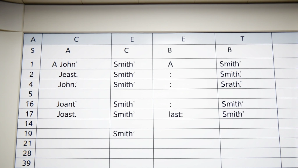
How to Merge Two Columns in Excel: Simple & Essential Tips

Merging columns in Excel is one of the most practical skills you’ll learn when working with spreadsheets. Whether you’re combining first and last names, joining addresses, or consolidating data from multiple sources, knowing how to merge two columns in Excel can save you hours of manual work. This guide walks you through every method—from simple formulas to advanced techniques—so you can choose the approach that works best for your situation.

• Merge Cells (visual merging for formatting)
• Concatenation Formula Method (recommended for data)
• CONCATENATE Function
• TEXTJOIN Function (modern Excel)
• Flash Fill Feature (Excel 2013+)
• Power Query Method (advanced)
• Combining with Delimiters and Separators
• Troubleshooting Common Issues

Understanding Merge Cells vs. Combining Data

Before learning how to merge two columns in Excel, it’s critical to understand the difference between merging cells and combining data. Many users confuse these two operations, which serve completely different purposes. Merging cells is a formatting operation that combines the appearance of multiple cells into one, while combining data actually joins the content from two columns into a single cell.

When you merge cells visually, Excel combines them into a single larger cell. This is purely cosmetic and doesn’t actually combine the data—it only keeps the content from the top-left cell and discards the rest. This approach is useful for headers or labels but problematic for data consolidation. Combining data, on the other hand, preserves all information from both columns and creates new content by joining them together.

For most practical purposes, combining data from two columns is what you actually need. This preserves your original information and creates a new merged result. According to WikiHow’s comprehensive guides, the formula-based approach is the industry standard for professional spreadsheet work because it maintains data integrity and allows for easy updates.

Key differences:

• Merge Cells: Formatting only; combines cell appearance; loses data from non-primary cells
• Combine Data: Preserves all information; creates new merged content; uses formulas
• Best for: Data consolidation, names, addresses, and any scenario where you need all information preserved

Using the Concatenation Formula (&) Method

The ampersand (&) method is the simplest and most reliable way to merge two columns in Excel. This concatenation operator joins text from multiple cells into one, and it’s been the standard approach for decades. To use this method, you’ll create a formula in a new column that references the two columns you want to combine.

Step-by-step process:

1. Click on an empty column where you want the merged data to appear (typically column C if merging A and B)
2. Click on the first cell in that column (C1)
3. Type the formula: =A1&" "&B1 (the space in quotes adds a space between the values)
4. Press Enter to confirm the formula
5. Click back on cell C1 and copy the formula down to all rows with data
6. Select all the merged results, copy them, then paste as values into a new location if desired

This method works beautifully for combining first and last names, street addresses with cities, or any two-column data. The space between the ampersands (" ") ensures your merged data is readable. You can customize this separator to use commas, hyphens, or any other character.

The beauty of the ampersand method is its flexibility. You can easily modify the formula to add different separators, adjust spacing, or include additional columns. Many Excel professionals prefer this approach because it’s transparent—anyone looking at your formula can immediately understand what’s happening.

The CONCATENATE Function Explained

Before the ampersand method became dominant, Excel users relied on the CONCATENATE function to merge columns. While older, this function still works perfectly and some users find it more intuitive. The CONCATENATE function takes multiple text values as arguments and joins them together into a single string.

Basic syntax:

=CONCATENATE(A1," ",B1)

This formula produces identical results to the ampersand method but uses a more explicit function call. If you’re merging three or more columns, CONCATENATE can actually be clearer than chaining multiple ampersands together. For example, =CONCATENATE(A1," ",B1," ",C1) is arguably more readable than =A1&" "&B1&" "&C1.

The main limitation of CONCATENATE is that it doesn’t handle arrays as efficiently as newer functions. If you’re working with large datasets or need advanced text manipulation, the newer TEXTJOIN function offers superior performance and features. However, for straightforward merging of two columns, CONCATENATE remains reliable and widely supported across all Excel versions.

TEXTJOIN: The Modern Solution

Introduced in Excel 2016, the TEXTJOIN function represents the modern standard for how to merge two columns in Excel. This powerful function combines the simplicity of concatenation with advanced features like automatic delimiter handling and the ability to ignore empty cells. TEXTJOIN is particularly valuable when working with variable-length data or when you need to merge multiple columns efficiently.

TEXTJOIN syntax:

=TEXTJOIN(" ",TRUE,A1:B1)

The three arguments work as follows: the first specifies your delimiter (space, comma, etc.), the second tells Excel whether to ignore empty cells (TRUE = yes, FALSE = no), and the third is the range of cells to combine. This approach is significantly more elegant than chaining multiple ampersands or using CONCATENATE.

TEXTJOIN’s true power emerges when merging multiple columns or handling inconsistent data. The function automatically applies your delimiter between all values, eliminating the need to manually specify separators for each cell reference. It also intelligently skips empty cells when you set the second parameter to TRUE, preventing awkward spacing issues in your merged results.

If you’re using Excel 2016 or later, TEXTJOIN should be your go-to function for merging columns. It’s faster to write, more readable, and handles edge cases better than older methods. According to The Spruce’s technical resources, TEXTJOIN has become the preferred method among Excel professionals for its reliability and flexibility.

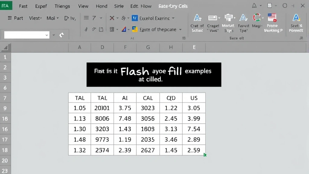
Flash Fill: Automatic Column Merging

Flash Fill is an intelligent Excel feature that automatically detects patterns in your data and fills in remaining cells accordingly. Available in Excel 2013 and later, Flash Fill can recognize when you’re merging two columns and automatically complete the task for you. This method requires no formulas and works through pattern recognition, making it ideal for users who prefer visual workflows.

How to use Flash Fill for merging:

1. In your destination column (C1), manually type the merged result for the first row (e.g., “John Smith” if merging “John” and “Smith”)
2. Move to C2 and type the merged result for the second row
3. Excel will often suggest the pattern automatically
4. Press Ctrl+E to activate Flash Fill, or go to Data > Flash Fill
5. Excel fills the remaining cells based on the detected pattern

Flash Fill works remarkably well for straightforward merging tasks, but it has limitations. It struggles with complex patterns, inconsistent formatting, or when your data contains exceptions. Additionally, Flash Fill creates static results rather than formulas, meaning if your source data changes, your merged column won’t automatically update.

For this reason, Flash Fill is best used for one-time data consolidation projects rather than ongoing spreadsheets. If you need dynamic updating when source data changes, stick with formula-based methods. However, for quick merging tasks where you don’t need formula flexibility, Flash Fill is remarkably efficient and requires zero technical knowledge.

Power Query for Advanced Merging

Power Query is Excel’s advanced data transformation tool, available in Excel 2010 and later (as an add-in) or built-in to Excel 2016+. For complex merging scenarios involving large datasets, data cleaning, or multiple transformation steps, Power Query provides professional-grade capabilities. This method is more technical but incredibly powerful for enterprise-level spreadsheet work.

Power Query allows you to merge columns while simultaneously performing other data operations like filtering, sorting, or removing duplicates. You can also save your query steps, meaning they’ll automatically apply to new data imported into your spreadsheet. This makes Power Query ideal for recurring data consolidation tasks.

Basic Power Query merging steps:

1. Select your data range and go to Data > From Table/Range
2. In the Power Query Editor, select both columns you want to merge
3. Right-click and choose “Merge Columns”
4. Specify your separator and column name
5. Click “OK” and then “Close & Load” to apply changes

While Power Query has a steeper learning curve than simple formulas, it’s invaluable for professional data work. If you’re regularly working with large Excel files or need to automate data consolidation, investing time in learning Power Query pays dividends. For most users, however, the TEXTJOIN or ampersand methods provide sufficient functionality without the complexity.

Working with Delimiters and Separators

When you merge two columns in Excel, choosing the right delimiter—the character separating your values—significantly impacts readability and usability. Common delimiters include spaces, commas, hyphens, slashes, and pipes. Your choice depends on your data type and how you plan to use the merged results.

Common delimiter examples:

• Space: =A1&" "&B1 – Best for names (“John Smith”)
• Comma + Space: =A1&", "&B1 – Good for lists (“Smith, John”)
• Hyphen: =A1&"-"&B1 – Useful for codes or IDs (“ABC-123”)
• Slash: =A1&"/"&B1 – Common for dates or fractions (“01/15/2024”)
• Pipe: =A1&"|"&B1 – Professional for data exports (“Data1|Data2”)

You can also use no delimiter at all by removing the separator parameter: =A1&B1. This directly concatenates values without spacing, useful for creating product codes or identifiers. The key is consistency—choose one delimiter style and apply it throughout your spreadsheet for professional appearance and easier downstream processing.

When using TEXTJOIN, you specify the delimiter as the first argument, making it easy to experiment with different separators. Try different options with a small sample of your data before applying to your entire dataset. You can also use special characters like line breaks (CHAR(10)) for advanced formatting, though these work best when combined with text wrapping—which you can learn more about in our guide on how to wrap text in Excel.

Troubleshooting and Best Practices

Even experienced users encounter issues when merging columns in Excel. Understanding common problems and their solutions ensures your data consolidation projects run smoothly. The most frequent issues involve formula errors, unexpected results, or data loss when improperly using the Merge Cells feature.

Common problem: #VALUE! error

This error typically occurs when your formula tries to concatenate cells containing errors or incompatible data types. Solution: Use IFERROR to handle problematic cells: =IFERROR(A1&" "&B1,""). This returns a blank cell instead of an error if something goes wrong.

Common problem: Unwanted spaces or formatting

If your merged results have extra spaces, use the TRIM function to clean them: =TRIM(A1&" "&B1). TRIM removes leading and trailing spaces, creating cleaner results. This is especially important when your source data has inconsistent spacing.

Common problem: Data loss when using Merge Cells

If you accidentally used the visual Merge Cells feature, you’ve lost data from all but the first cell. Always use formula-based merging instead. The how to create a drop down list in Excel guide demonstrates how to work with merged cells safely in other contexts.

Best practices for merging columns:

• Always work in a new column: Never overwrite your original data in case you need to reverse the operation
• Use formulas, not visual merging: Formulas preserve data and allow updates; visual merging loses information
• Test with a few rows first: Verify your formula produces correct results before copying to thousands of rows
• Convert to values when done: Once satisfied, copy your merged column and paste as values to reduce file size and formula complexity
• Document your process: Add a comment or note explaining your merge formula for future reference
• Keep originals intact: Maintain your original columns in case you need to make adjustments later

According to Family Handyman’s practical approach to DIY projects, the same principle applies to data work: preparation and documentation prevent problems. Taking time to set up your merge properly saves debugging time later.

When working with large datasets, performance matters. TEXTJOIN and the ampersand method are fastest for most scenarios. CONCATENATE is slightly slower but still acceptable. Flash Fill is quickest for one-time tasks but can’t handle complex patterns. Power Query is best for recurring, complex operations on massive datasets.

If you’re frequently manipulating spreadsheet layouts and structures, you might also benefit from learning how to freeze panes in Excel to keep headers visible while working, or how to lock a row in Excel to protect important data. These complementary skills make you more efficient with spreadsheet work overall.

FAQ

Q: Does merging columns delete my original data?

A: No, not if you use formula-based merging. Your original data remains in columns A and B; the merged result appears in column C. Only the visual Merge Cells feature causes data loss, which is why formula-based approaches are recommended.

Q: Can I merge more than two columns?

A: Absolutely. Extend any formula by adding more ampersands or cell references. For example: =A1&" "&B1&" "&C1 merges three columns. TEXTJOIN handles this elegantly: =TEXTJOIN(" ",TRUE,A1:C1).

Q: What’s the difference between CONCATENATE and the ampersand method?

A: They produce identical results. The ampersand method is simpler and faster to type. CONCATENATE is more explicit and some find it clearer. Choose whichever feels more natural; both are perfectly valid.

Q: Why should I convert merged formulas to values?

A: Converting to values reduces file size, speeds up calculations, and breaks the link to original columns. This is useful when you’re done editing and want a final, static result. Copy your merged column, then Paste Special > Values.

Q: Does TEXTJOIN work in older Excel versions?

A: No, TEXTJOIN was introduced in Excel 2016. If you’re using Excel 2013 or earlier, use the ampersand method or CONCATENATE function instead. Check your Excel version in File > Account > About Excel.

Q: Can I undo a merge if I make a mistake?

A: Yes, press Ctrl+Z immediately after merging to undo. If you’ve already saved, you’ll need to manually recreate your original data or restore from a backup. Always save before major operations as a precaution.

Q: How do I merge columns without creating a new column?

A: Create your merged data in a temporary column, then copy and paste the values back into your original column. However, this overwrites your original data, so only do this if you’ve backed up your file first.

Q: What if my columns contain numbers instead of text?

A: Excel automatically converts numbers to text when concatenating. However, formatting may be lost (like currency symbols or decimal places). Use TEXT function for control: =TEXT(A1,"$0.00")&" "&B1.

Q: Can I merge columns in Excel Online?

A: Yes, Excel Online supports the ampersand method, CONCATENATE, and TEXTJOIN functions. Flash Fill and Power Query are not available in the web version, but formula-based merging works identically.

For additional guidance on Excel techniques, HowStuffWorks offers excellent technical tutorials covering spreadsheet fundamentals. Whether you’re learning how to unhide all rows in Excel or mastering advanced merging techniques, these resources support your learning journey. You can also explore how to freeze a row in Excel for better data organization alongside your column merging work.