How to Freeze Cells in Excel: Essential Easy Guide

Working with large spreadsheets in Excel can be frustrating when you scroll down and lose sight of your column headers. Learning how to freeze cells in Excel is one of the most valuable productivity skills you can master. Whether you’re managing a budget, tracking inventory, or analyzing sales data, freezing rows and columns keeps your reference headers visible while you navigate through hundreds of rows of data. This guide walks you through every method to freeze cells in Excel, from basic freezing techniques to advanced multi-pane setups.

Quick Answer

To freeze cells in Excel quickly, select the cell below and to the right of what you want to freeze, then click the View tab and select Freeze Panes. For example, to freeze the first row and first column, click cell B2, then choose Freeze Panes. To unfreeze, return to the View tab and click Unfreeze Panes. This method works identically across Excel desktop versions and Excel Online.

Tools & Materials

• Microsoft Excel (Desktop version 2016 or later, or Excel Online)
• A spreadsheet with headers or data you want to keep visible
• Mouse or trackpad for clicking menu options
• Optional: External monitor for easier navigation of large datasets

How to Freeze the First Row in Excel

Freezing the first row is the most common use case for how to freeze cells in Excel. This keeps your column headers visible while scrolling through data below. The process is straightforward and takes just two clicks.

Step 2: Access the View Tab. Navigate to the ribbon at the top of Excel and click the View tab. This opens the viewing options menu where freeze pane controls are located.

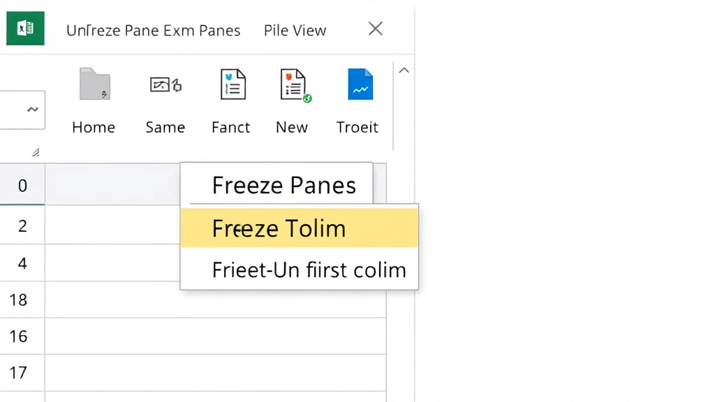
Step 3: Select Freeze Panes. In the View tab, locate the Freeze Panes button (usually in the upper-left section). Click it, and a dropdown menu appears with three options: Freeze Panes, Freeze Top Row, and Freeze First Column.

Step 4: Choose Your Option. Click Freeze Top Row for the quickest method. Excel immediately freezes row 1, and you’ll see a subtle line separating the frozen row from the scrollable content below. Now when you scroll down through your data, the header row stays locked at the top.

Verification: Test your freeze by scrolling down. Your first row should remain visible while the rest of the spreadsheet moves. You’ve successfully frozen your first row and can now navigate large datasets without losing context.

How to Freeze the First Column

Sometimes you need to keep the first column visible while scrolling horizontally across many columns. This is especially useful when your first column contains item names, product codes, or identifiers that you want to reference while viewing data to the right.

Step 1: Click on Column B. Select any cell in the second column (B1, B2, or any B cell). This designates everything to the left as the frozen area.

Step 2: Open the View Tab. Click View in the ribbon menu at the top of your screen.

Step 3: Click Freeze Panes. In the View tab, click the Freeze Panes button and select Freeze First Column from the dropdown menu. Excel applies the freeze immediately.

Test Horizontal Scrolling: Use the horizontal scroll bar at the bottom of your spreadsheet to scroll right. Your first column remains anchored to the left side while other columns move. This technique is invaluable when working with wide datasets containing many columns of information.

You can also learn more about column-specific freezing by checking our guide on how to freeze a row in Excel, which covers related techniques.

How to Freeze Multiple Rows and Columns Simultaneously

The most powerful application of how to freeze cells in Excel involves freezing both rows and columns at the same time. This creates a locked pane in the top-left corner while allowing you to scroll both vertically and horizontally.

Step 1: Select Your Anchor Cell. Click the cell that sits below and to the right of all the rows and columns you want to freeze. For example, if you want to freeze the first two rows and first three columns, click cell D3. This cell becomes your reference point—everything above and to the left will freeze.

Step 2: Navigate to View Tab. Click the View tab in the Excel ribbon.

Step 3: Click Freeze Panes. In the View tab, click Freeze Panes (not the dropdown arrow, but the button itself). Excel analyzes your selection and freezes everything above and to the left of your chosen cell.

Visible Indicators: You’ll notice thin black lines appearing on your spreadsheet—one horizontal line below your frozen rows and one vertical line to the right of your frozen columns. These lines show exactly where the freeze boundaries are located.

Practical Example: Imagine a sales spreadsheet with months across the top (columns) and product names down the left side (rows). By selecting cell B2, you freeze the month headers and product names, allowing you to view any combination of data while always knowing which product and month you’re examining.

For more advanced row-freezing techniques, visit our article on how to pin a row in Excel.

” alt=”Excel spreadsheet showing freeze panes dividing lines between frozen and scrollable sections”>

Freeze Panes vs. Split Windows: Understanding the Difference

Excel offers two similar but distinct features: Freeze Panes and Split Windows. Understanding the difference helps you choose the right tool for your task. Freeze Panes locks specific rows and columns in place while you scroll, whereas Split Windows creates independent scrollable panes that you control separately.

Freeze Panes Characteristics: When you freeze panes, the frozen areas remain fixed while other sections scroll. You have one active scroll position—when you scroll down, the entire unfrozen area moves together. The frozen sections don’t scroll independently. This is ideal for keeping headers visible while viewing data.

Split Windows Characteristics: The Split feature divides your spreadsheet into separate panes that scroll independently. You can view row 1 in the top pane while simultaneously viewing row 500 in the bottom pane, each with independent scroll bars. This is useful when comparing data from different parts of your spreadsheet side-by-side.

Choosing Between Them: Use Freeze Panes for standard header-locking scenarios. Use Split Windows when you need to compare non-adjacent sections of your data simultaneously. Most users find Freeze Panes sufficient for daily work, but Split Windows offers flexibility for complex analysis tasks.

How to Unfreeze Cells in Excel

Removing a freeze is just as simple as creating one. Whether you’ve changed your data structure or want to try a different freezing configuration, unfreezing takes seconds.

Step 1: Click the View Tab. Open the View tab in your Excel ribbon.

Step 2: Click Freeze Panes. In the View tab, click the Freeze Panes button to reveal the dropdown menu.

Step 3: Select Unfreeze Panes. The dropdown menu shows an Unfreeze Panes option at the top. Click it, and Excel immediately removes all frozen panes from your spreadsheet. The black dividing lines disappear, and your spreadsheet returns to normal scrolling behavior.

Verification: After unfreezing, scroll through your spreadsheet to confirm that all sections scroll together without any locked areas. You can now reapply freezing with different settings if needed.

Freezing Cells in Excel Online

Excel Online provides the same how to freeze cells in Excel functionality as the desktop version, though the interface differs slightly. If you work with cloud-based Excel files, these steps apply to your workflow.

Step 1: Select Your Freeze Point. Click the cell below and to the right of the rows and columns you want to freeze, just as you would in desktop Excel.

Step 2: Access the View Menu. Click the View tab in the Excel Online ribbon. The menu layout is similar to desktop Excel but may appear slightly different depending on your browser and screen size.

Step 3: Click Freeze Panes. Look for the Freeze Panes option in the View menu. Click it to access freeze options.

Step 4: Select Your Freeze Type. Choose from Freeze Panes, Freeze Top Row, or Freeze First Column, depending on your needs. Excel Online applies the freeze immediately.

Compatibility Note: Freezes created in Excel Online remain intact when you open the file in desktop Excel, and vice versa. This makes freezing reliable across all Excel platforms, whether you work on Windows, Mac, or through a web browser.

Common Issues and Troubleshooting

Issue: Freeze Panes button appears grayed out. This usually means you’re on a sheet with very limited data or your selection is invalid. Ensure you’ve selected a cell that’s not in the first row or first column. Try clicking cell B2 and attempting to freeze again.

Issue: You froze the wrong rows or columns. Simply unfreeze using the steps above, then reselect your anchor cell and reapply the freeze. There’s no limit to how many times you can adjust your freeze settings.

Issue: Frozen panes aren’t scrolling as expected. Verify that you’re scrolling in the unfrozen area of your spreadsheet. Click within the scrollable section (below or to the right of the freeze lines) before using scroll bars. Sometimes clicking the frozen area prevents scrolling.

Issue: Freeze Panes disappeared after saving. This is rare but can happen with corrupted files. Try unfreezing, saving, closing, and reopening your file. Then reapply your freeze settings.

According to WikiHow, freezing panes is one of Excel’s most underutilized features that dramatically improves spreadsheet navigation. As reviewed by Family Handyman in their productivity guides, mastering Excel features like freezing significantly reduces data entry errors and improves workflow efficiency.

You might also find our guide on how to create a dropdown in Excel helpful for building more sophisticated spreadsheets with frozen headers and data validation.

FAQ

Q: Can I freeze more than one row and one column at the same time?
A: Yes, absolutely. Select the cell below and to the right of all rows and columns you want to freeze. For example, to freeze the first three rows and first two columns, click cell C4, then apply Freeze Panes. Everything above row 4 and to the left of column C remains frozen.

Q: Does freezing affect printing?
A: No. When you print your spreadsheet, frozen panes don’t appear in the printed output. All rows and columns print normally without freeze indicators. This is helpful because it means your freeze settings are purely for on-screen navigation.

Q: Can I freeze panes in Excel on a Mac?
A: Yes. The process is identical on Mac. Click the cell where you want the freeze to begin, go to the View tab, and click Freeze Panes. Mac Excel uses the same interface and functionality as Windows Excel.

Q: What’s the difference between freezing and hiding rows?
A: Freezing keeps rows visible and locked in place while you scroll. Hiding removes rows from view entirely. If you want to hide rows instead, right-click the row number and select Hide. For unhiding information, check our guide on how to unhide all rows in Excel.

Q: Can I freeze panes in a shared Excel file?
A: Yes. Freeze settings are personal to your view and don’t affect other users’ views of the same file. Each person can set their own freeze preferences without impacting others working on the document.

Q: How many panes can I freeze at once?
A: You can freeze up to one horizontal line (separating rows) and one vertical line (separating columns) simultaneously. This creates four panes maximum: top-left (frozen), top-right (scrolls horizontally), bottom-left (scrolls vertically), and bottom-right (scrolls both directions).

Q: Will my freeze settings save when I close Excel?
A: Yes. Your freeze settings are saved with your file. When you reopen the spreadsheet, the same rows and columns remain frozen. This makes freezing a persistent feature that survives closing and reopening.

Q: Can I use freeze panes with filtered data?
A: Yes. Freezing and filtering work together seamlessly. You can freeze your header row and then apply filters to your data. The frozen header remains visible while you work with filtered results. For more on data organization, see our article on how to wrap text in Excel.

Q: Is there a keyboard shortcut for freezing panes?
A: Excel doesn’t have a built-in keyboard shortcut for Freeze Panes in most versions. You must use the View menu. However, you can create a custom keyboard shortcut through Excel’s macro settings if you freeze frequently.

As noted by Consumer Reports in their productivity software analysis, Excel’s freeze functionality is essential for professional data management. Additionally, The Spruce recommends freezing panes for anyone managing household budgets or inventory spreadsheets.

Mastering how to freeze cells in Excel transforms your spreadsheet experience from frustrating to efficient. Whether you’re managing a small budget or analyzing enterprise-level data, these techniques keep your headers visible and your workflow smooth. Start with freezing your first row, experiment with multiple panes, and soon you’ll wonder how you ever worked without this essential Excel feature.