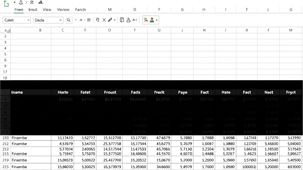
How to Pin a Row in Excel: Simple & Essential Guide

Pinning a row in Excel keeps your header row visible while scrolling through large datasets. This essential feature saves time and prevents confusion when working with spreadsheets containing hundreds or thousands of rows. Whether you’re managing sales data, inventory lists, or financial reports, knowing how to pin a row in Excel is a game-changer for productivity and data clarity.
Quick Answer: To pin a row in Excel, click on the row number below the row you want to pin, then go to the View tab and select “Freeze Panes.” This locks the selected row(s) in place while you scroll down, keeping column headers visible at all times. The process takes seconds and works identically across Excel versions on Windows and Mac.
Tools & Materials You’ll Need
- Microsoft Excel (2016 or newer, or Excel Online)
- A spreadsheet with data and headers
- Mouse or trackpad for navigation
- Optional: Multiple monitor setup for easier viewing
Understanding Row Pinning vs. Freezing Panes
Many users confuse “pinning” with “freezing panes,” but they’re essentially the same feature in Excel. When you pin a row, you’re freezing it in place so it remains visible while scrolling. This prevents your header row from disappearing when you navigate through large datasets. The terminology varies slightly depending on your Excel version, but the functionality is identical.
Pinning rows is different from simply selecting or hiding rows. When you pin a row in Excel, you create a visual dividing line that separates frozen content from scrollable content. This is particularly useful for spreadsheets with many columns and rows, where losing sight of headers creates confusion and errors.
According to WikiHow, freezing panes is one of the most underutilized Excel features, yet it dramatically improves workflow efficiency. Understanding this distinction helps you choose the right tool for your data management needs.
Step-by-Step: How to Pin a Row in Excel
Step 1: Open Your Spreadsheet
Launch Microsoft Excel and open the spreadsheet containing the row you want to pin. Ensure your data is organized with headers in the first row and data below. This is the standard format for pinning rows effectively.
Step 2: Select the Row Below Your Header
Click on the row number of the row immediately below the header row you want to pin. For example, if your headers are in Row 1, click on Row 2. This selection tells Excel which content should remain frozen and which should scroll.
Step 3: Access the View Tab
Navigate to the View tab in the Excel ribbon at the top of your screen. This tab contains all freezing and panning options for your spreadsheet.
Step 4: Click “Freeze Panes”
In the View tab, locate the “Freeze Panes” button. Click on it, and a dropdown menu appears with three options: “Freeze Panes,” “Freeze Top Row,” and “Unfreeze Panes.” Select “Freeze Panes” to pin your chosen row.
Step 5: Verify the Pin
After clicking “Freeze Panes,” notice the thin black line appearing below your selected row. This line indicates that the row above it is now pinned. Scroll down to confirm your header row remains visible while the rest of the data moves.

As detailed in our guide on how to freeze a row in Excel, this process works seamlessly across all modern Excel versions and provides immediate visual feedback.
Pinning Multiple Rows at Once
You’re not limited to pinning just one row in Excel. Many spreadsheets benefit from pinning multiple rows, such as when you have a title row, a subtitle row, and column headers. To pin multiple rows, select the row number below the last row you want to freeze.
For example, if you want to pin Rows 1, 2, and 3, click on Row 4, then go to View > Freeze Panes. This freezes all three rows above your selection, keeping them visible while you scroll through your data. This technique is invaluable when working with complex reports that include summary information at the top.
The same principle applies when pinning columns alongside rows. If you want to pin both the first column (often containing row labels) and the first three rows (headers), click on cell B4 and then select Freeze Panes. This creates both horizontal and vertical frozen sections, allowing you to navigate large datasets without losing context.
Unfreezing and Removing Pinned Rows
Removing a pinned row is just as simple as creating one. Return to the View tab and click “Freeze Panes” again. Instead of a dropdown menu, you’ll see the “Unfreeze Panes” option directly available. Click it to remove all frozen rows and columns from your spreadsheet.
This action removes the black dividing lines and allows your entire spreadsheet to scroll normally. You might unfreeze rows when sharing the spreadsheet with colleagues who prefer different viewing preferences, or when your data structure changes and headers are no longer necessary.
It’s worth noting that unfreezing affects the entire spreadsheet at once—you cannot unfreeze individual rows while keeping others frozen. If you need different freezing configurations, you’ll need to unfreeze, reorganize your data, and refreeze with new selections.
Advanced Pinning Techniques
Using Split Panes for Enhanced Navigation
Beyond basic pinning, Excel offers “Split Panes,” a related feature that divides your spreadsheet into separate scrollable sections. Unlike freezing, split panes allows each section to scroll independently. Access this through View > Split. This is particularly useful for comparing data in different sections of a large spreadsheet.
Pinning in Excel Online
If you’re using Excel Online (Excel on the web), the process is slightly different but equally straightforward. Open your spreadsheet, select the row below where you want to freeze, and use the same View > Freeze Panes option. Excel Online supports all the same pinning functionality as the desktop version.
Combining Pinning with Cell Locking
For additional data protection, combine pinning with cell locking. As explained in our article on how to lock cells in Excel, you can freeze rows while simultaneously protecting specific cells from editing. This creates a professional, secure spreadsheet environment.
Pinning Rows in Shared Workbooks
When sharing Excel files with colleagues, your pinned rows remain frozen for all users who open the file. This ensures consistent data presentation across your team. However, each user can modify the freeze settings for their own view without affecting others’ copies.
Troubleshooting Common Issues
Freeze Panes Option Appears Grayed Out
If the Freeze Panes button is unavailable, you likely have a filtered view or protected sheet active. Disable any active filters by going to Data > Filter > Toggle Filter, or unprotect your sheet through the Review tab. Once these are cleared, Freeze Panes becomes available.
Pinned Rows Scroll When They Shouldn’t
This typically occurs when you’ve selected the wrong row before freezing. Remember, you must click the row number below the rows you want to freeze. If your freeze isn’t working correctly, unfreeze completely, then reselect and freeze the proper row.
Black Line Not Appearing After Freezing
The dividing line is subtle on some displays. Scroll down slightly—the frozen rows should remain at the top while your data moves. The black line may not be immediately visible, but the functionality is still active.
Printing Issues with Frozen Rows
By default, frozen rows don’t print on every page. To print headers on every page, use the Page Layout tab and set Print Titles under Sheet Options. This ensures your frozen headers appear on all printed pages, not just the first one.
Best Practices for Data Organization
To maximize the benefits of pinning rows in Excel, organize your data strategically. Keep headers in the first row, use consistent formatting, and avoid merging cells in header rows—merged cells can complicate freezing behavior.
When working with large datasets, consider using tables instead of regular ranges. Excel tables include built-in headers and automatically adjust when you add or remove data. You can still pin table headers using the same Freeze Panes method, and the functionality integrates seamlessly.
For spreadsheets with multiple sections or summaries, use clear visual separation between sections. This makes it obvious where frozen rows end and scrollable content begins, reducing user confusion. Color-coding headers also helps users quickly identify pinned rows.
According to The Spruce, proper spreadsheet organization saves time and reduces errors in data entry and analysis. Pinning rows is just one component of a well-organized Excel workflow.
When collaborating on spreadsheets, establish team standards for pinning. Consistent freezing practices across all shared files make navigation intuitive for everyone. Document these standards in your team’s Excel guidelines or training materials.
Additionally, consider using how to find duplicates in Excel techniques alongside pinning to maintain data quality. Pinned headers help you spot duplicates more easily since you always see your column labels.
FAQ
Q: Can I pin rows in Google Sheets?
A: Yes, Google Sheets has a “Freeze” feature that works similarly to Excel. Right-click on the row number and select “Freeze,” or use the Data menu to access freeze options. The functionality is nearly identical to Excel’s pinning feature.
Q: Will pinned rows remain frozen when I save and reopen the file?
A: Absolutely. Excel saves your freeze settings with the file. When you or anyone else opens the spreadsheet later, the pinned rows remain frozen exactly as you configured them.
Q: Can I pin rows and columns simultaneously?
A: Yes. Select the cell at the intersection of where you want to freeze (for example, cell B2 to freeze Row 1 and Column A). Then apply Freeze Panes, and both will remain frozen while you scroll.
Q: What’s the maximum number of rows I can pin?
A: Technically, you can freeze any number of rows, but practically, freezing more than 5-10 rows reduces your visible data area. Most users find pinning 1-3 rows optimal for data visibility and navigation.
Q: Does pinning rows affect printing?
A: Pinned rows print normally on the first page, but they don’t automatically repeat on subsequent pages. Use Print Titles in the Page Layout tab to repeat headers on every printed page.
Q: Can I pin rows in Excel for Mac?
A: Yes, the process is identical. Go to View > Freeze Panes and select your desired option. Mac users have full access to all pinning and freezing features.
Q: What happens if I delete a pinned row?
A: If you delete a pinned row, the freeze remains at the same position. The next row becomes the new frozen row. If you delete rows below the freeze line, the freeze position doesn’t change.
Learning how to pin a row in Excel is fundamental to efficient spreadsheet management. This simple yet powerful feature transforms how you work with large datasets, keeping critical information visible while you navigate through your data. Whether you’re managing financial reports, inventory lists, or research data, mastering row pinning ensures accuracy and productivity. As referenced by Family Handyman, organization and accessibility are key to any successful project, and the same applies to Excel spreadsheet management.


